3Making Light Work in BiologyBasic, Foundational Detection and Imaging Techniques Involving Ultraviolet, Visible, and Infrared Electromagnetic Radiation Interactions with Biological Matter
I don’t suppose you happen to know
Why the sky is blue?…
Look for yourself. You can see it’s true.
—John Ciardi (American poet 1916–1986)
General Idea: Here, we discuss the broad range of experimental biophysical techniques that primarily act through the detection of biological components using relatively routine techniques, which utilize basic optical photon absorption and emission processes and light microscopy, and similar methods that extend into the ultraviolet (UV) and infrared (IR) parts of the electromagnetic spectrum. These include methods to detect and image cells and populations of several cells, as well as subcellular structures, down the single-molecule level both for in vitro and in vivo samples. Although the techniques are ubiquitous in modern biophysics labs, they are still robust, have great utility in addressing biological questions, and have core physics concepts at their heart that need to be understood.
3.1 Introduction
Light microscopy, invented over 300 years ago, has revolutionized our understanding of biological processes. In its modern form, it involves much more than just the magnification of images in biological samples. There are invaluable techniques that have been developed to increase the image contrast. Fluorescence microscopy, in particular, is a very useful tool for probing biological processes. It results in high signal-to-noise ratios (SNRs) for determining the localization of biological molecules tagged with a fluorescent dye but does so in a way that is relatively noninvasive. This minimal perturbation to the native biology makes it a tool of choice in many biophysical investigations.
There has been enormous development of visible (VIS) light microscopy tools, which address biological questions at the level of single cells in particular, due in part to a bidirectional development in the operating range of sample length scales over recent years. Top-down improvements in in vivo light microscopy technologies have reduced the scale of spatial resolution down to the level of single cells, while bottom-up optimization of many emerging single-molecule light microscopy methods originally developed for in vitro contexts has been applied now to living cells.
3.2 Basic UV-VIS-IR Absorption, Emission, and Elastic Light Scattering Methods
Before we discuss the single-molecule light microscopy approaches, there are a number of basic spectroscopy techniques that are applied to bulk in vitro samples, which not only primarily utilize VIS light but also extend into UV and IR. Some of these may appear mundane at first sight, but in fact they hold the key to generating many preliminary attempts at robust physical quantification in the biosciences.
3.2.1 Spectrophotometry
In essence, a spectrophotometer (or spectrometer) is a device containing a photodetector to monitor the transmittance (or conversely the reflectance) of light through a sample as a function of wavelength. Instruments can have a typical wavelength range from the long UV (~200–400 nm) through to the VIS (~400–700 nm) up into the mid and far IR (~700–20,000 nm) generated from one or more broadband sources in combination with wavelength filters and/or monochromators. A monochromator uses either optical dispersion or diffraction in combination with mechanical rotation to select different wavelengths of incident light. Light is then directed through a solvated sample that is either held in a sample cuvette or sandwiched between transparent mounting plates. They are generally made from glass or plastic for VIS, sodium chloride for IR, or quartz for UV to minimize plate/cuvette absorption at these respective wavelengths. Incident light can be scanned over a range of wavelengths through the sample to generate a characteristic light absorption spectral response.
Scanning IR spectrophotometers exclusively scan IR wavelengths. A common version of this is the Fourier transform infrared (FTIR) spectrometer, which, instead of selecting one probe wavelength at any one time as with the scanning spectrophotometer, utilizes several in one go to generate a polychromatic interference pattern from the sample, which has some advantage in terms of SNR and spectral resolution.
The absorption signal can then be inverse Fourier transformed to yield the IR absorption spectrum. Such spectra can be especially useful for identifying different organic chemical motifs in samples, since the vibrational stretch energy of the different covalent bonds found in biomolecules corresponds to IR wavelengths and will be indicated by measurable absorption peaks in the spectrum. The equivalent angular frequency for IR absorption, ω, can be used to estimate the mean stiffness of a covalent bond (a useful parameter in molecular dynamics simulations, see Chapter 8), by modeling it as a simple harmonic oscillator of two masses m1 and m2 (representing the masses of the atoms either end of the bond) joined by a spring of stiffness kr:
(3.1)where μ is the reduced mass given by
(3.2)Technical experts of IR spectrometers generally do not cite absorption wavelengths but refer instead to wavenumbers in units of cm−1, with the range ~700–4000 cm−1 being relevant to most of the different covalent bonds found in biomolecules, which corresponds to a wavelength range of ~2.5–15 μm. Although broadband IR sources are still sometimes used in older machines, it is more common now to use IR laser sources.
The pattern of IR absorption peaks in the spectrum, their relative position in terms of wavelength and amplitude, can generate a unique signature for a given biochemical component and so can be invaluable for sample characterization and purity analysis. The principal drawback of IR spectroscopy is that water exhibits an intense IR absorption peak and samples need to be in a dehydrated state. IR absorption ultimately excites a transition between different bond vibrational states in a molecule (Figure 3.1a), which implies a change in electrical dipole moment, due to either electrical polar asymmetry of the atoms that form the bond or the presence of delocalized electronic molecular orbitals (Table 3.1).
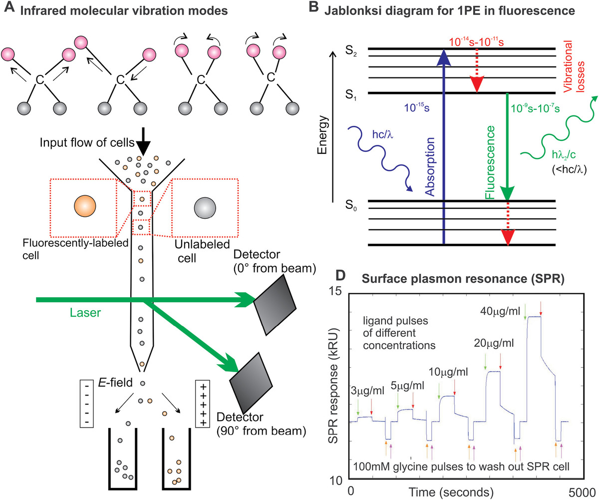
Figure 3.1 Simple spectroscopy and fluorescence excitation. (a) Some typical vibrational modes of a carbon atom–centered molecular motif that are excited by infrared absorption. (b) Jablonski energy level transition diagram for single-photon excitation resulting in fluorescence photon emission, characteristic time scales indicated. (c) Schematic of a typical fluorescence-assisted cell sorting device. (d) Typical output response from an SPR device showing injection events of a particular ligand, followed by washes and subsequent ligand injections into the SPR chamber of increasing concentration.
| Peak IR Absorption Range (cm−1) | Bond in Biomolecule |
|---|---|
| 730–770 | C—H |
| 1180–1200 | C—O—C |
| 1250–1340 | C—N |
| 1500–1600 | C=C |
| 1700–1750 | C=O |
| 2500–2700 (and other peaks) | O—H |
| 3300–3500 (and other peaks) | N—H |
Conventional FTIR is limited by a combination of factors including an inevitable trade-off between acquisition time and SNR and the fact that there is no spatial localization information. However, recent developments have utilized multiple intense, collimated IR beams from synchrotron radiation (see Chapter 5). This approach permits spatially extended detection of IR absorption signals across a sample allowing diffraction-limited time-resolved high-resolution chemical imaging, which has been applied to tissue and cellular samples (Nasse et al., 2011).
Many biomolecules that contain chemical bonds that absorb in the IR will also have a strong Raman signal. The Raman effect is one of the inelastic scattering of an excitation photon by a molecule, resulting in either a small increase or decrease in the wavelength of the scattered light. There is a rough mutual exclusion principle, in that strong absorption bands in the IR correspond to relatively weak bands in a Raman spectrum, and vice versa. Raman spectroscopy is a powerful biophysical tool for generating molecular signatures, discussed fully in Chapter 4.
Long UV light (~200–400 nm) is also a useful spectrophotometric probe especially for determining proteins and nucleic acid content in a sample. Peptide bonds absorb most strongly at ~280 nm wavelength, whereas nucleic acids such as RNA and DNA have a peak absorption wavelength of more like ~260 nm. It is common therefore to use the rate of absorption at these two wavelengths as a metric for protein and/or nucleic acid concentration. For example, a ratio of 260/280 absorbance of ~1.8 is often deemed as “pure” by biochemists for DNA, whereas a ratio of ~2.0 is deemed “pure” for RNA. If this ratio is significantly lower, it often indicates the presence of protein (or potentially other contaminants such as phenol that absorb strongly at or near 280 nm). With suitable calibration, however, the 260 and 280 nm absorption values can be used to determine the concentrations of nucleic acids and proteins in the absence of sample contaminants.
In basic spectrophotometers, the transmitted light intensity from the sample is amplified and measured by a photodetector, typically a photodiode. More expensive machines will include a second reference beam using an identical reference cuvette with the same solvent (generally water, with some chemicals to stabilize the pH) but no sample, which can be used as a baseline against which to reference the sample readings. This method finds utility in measuring sample density containing relatively large biological particulates (e.g., cells in suspension, to determine the so-called growth stage) to much smaller ones, such as molecules in solution.
To characterize attenuation, if we assume that the rate absorption of light parallel to the direction of propagation, say z, in an incrementally small slice through the sample is proportional to the total amount of material in that thin slice multiplied by the incident light intensity I(z), then it is trivial to show for a homogeneous tissue:
(3.3)This is called the “Beer–Lambert law,” a very simple model that follows from the assumption that the drop in light intensity upon propagating through a narrow slice of sample is proportional to the incident intensity and the slice’s width. It is empirically obeyed up to high scatterer concentrations beyond which electrostatic interactions between scatterers become significant. Here, σ is the mean absorption cross-sectional area of the tissue, which depends on the wavelength λ, and C is the concentration of the absorbing molecules. The absorbance A is often a useful quantity, defined as
(3.4)For a real tissue over a wide range of z, there may be heterogeneity in terms of the types of molecules, their absorption cross-sectional areas, and their concentrations. The Beer–Lambert law can be utilized to measure the concentration of a population of cells. This is often cited as the optical density (OD) measurement, such that
(3.5)where L is the total path length over which the absorbance measurement was made. Many basic spectrophotometers contain a cuvette, which is standardized at L = 1 cm, and so it is normal to standardize OD measurements on the assumption of a 1 cm path length.
Note that the absorbance measured from a spectrophotometer is not exclusively due to photon absorption processes as such, though photon absorption events may contribute to the reduction in transmitted light intensity, but rather scattering. In simple terms, general light scattering involves an incident photon inducing an oscillating dipole in the electron molecular orbital cloud, which then reradiates isotropically. The measured reduction in light intensity in passing through a biological sample in a standard VIS light spectrophotometer is primarily due to elastic scattering of the incident light. For scattering particles, the size of single cells is at least an order of magnitude greater than the wavelength of the incident light; this phenomenon is due primarily to Mie scattering. More specifically, this is often referred to as “Tyndall scattering”: Mie scattering in a colloidal environment in which the scattering particles may not necessarily be spherical objects. A good example is the rod-shaped bacteria cells. Differences in scatterer shape results in apparent differences in OD; therefore, caution needs to be applied in ensuring that like is compared to like in terms of scatterer shape when comparing OD measurements, and if not, then a shape correction factor should be applied. Note that some absorbance spectrometers are capable of correcting for scattering effects.
These absorbance measurements are particularly useful for estimating the density of growing microbial cultures, for example, with many bacteria an OD unit of 1.0 taken at a conventional wavelength of 600 nm corresponds to ~108 cells mL−1, equivalent to a typical cloudy looking culture when grown to “saturation.” Spectrophotometry can be extended into colorimetry in which an indicator dye is present in the sample, which changes color upon binding of a given chemical. This can then be used to report whether a given chemical reaction has occurred or not, and so monitoring the color change with time will indicate details of the kinetics of that chemical reaction.
3.2.2 Fluorimetry
A modified spectrophotometer called a fluorimeter (or fluorometer) can excite a sample with incident light over a narrow band of wavelengths and capture fluorescence emissions. For bulk ensemble average in vitro fluorimetry investigations, several independent physical parameters are often consolidated for simplicity into just a few parameters to characterize the sample. For example, the absorption cross-section for a fluorescent sample is related to its extinction coefficient ε (often cited in non-SI units of M−1 cm−1) and the molar concentration of the fluorophore cm by
(3.6)Therefore, the Beer–Lambert law for a fluorescent sample can be rewritten as
(3.7)The key physical process in bulk fluorimetry is single-photon excitation, that is, the processes by which energy from one photon of light is absorbed and ultimately emitted as a photon of lower energy. The process is easier to understand when depicted as a Jablonski diagram for the various energy level transitions involved (Figure 3.1b). First, the photon absorbed by the electron shells of an atom of a fluorophore (a fluorescent dye) causes an electronic transition to a higher energy state, a process that takes typically ~10−15 s. Vibrational relaxation due to internal conversion (in essence, excitation of an electron to a higher energy state results in a redistribution of charge in the molecular orbitals resulting in electrostatically driven oscillatory motion of the positively charged nucleus) relative movements can then occur over typically 10−12 to 10−10 s, resulting in an electronic energy loss. Fluorescence emission then can occur following an electronic energy transition back to the ground state over ca. 10−9 to 10−6 s, resulting in the emission of a photon of light of lower energy (and hence longer wavelength) than the excitation light due to the vibrational losses.
In principle, an alternative electronic transition involves the first excited triplet state energy level reached from the excited state via intersystem crossing in a classically forbidden transition from a net spin zero to a spin one state. This occurs over longer time scales than the fluorescence transition, ca. 10−3–100 s, and results in emission of a lower-energy phosphorescence photon. This process can cause discrete photon bunching over these time scales, which is not generally observed for typical data acquisition time scales greater than a millisecond as it is averaged out. However, there are other fluorescence techniques using advanced microscopy in which detection is performed over much faster time scales, such as fluorescence lifetime imaging microscopy (FLIM) discussed later in this chapter, for which this effect is relevant.
The electronic energy level transitions of ground-state electron excitation to excited state, and from excited state back to ground state, are vertical transitions on the Jablonski diagram. This is due to the quantum mechanical Franck–Condon principle that implies that the atomic nucleus does not move during these two opposite electronic transitions and so the vibration energy levels of the excited state resemble those of the ground state. This has implications for the symmetry between the excitation and emission spectra of a fluorophore.
But for in vitro fluorimetry, a cuvette of a sample is excited into fluorescence often using a broadband light source such as a mercury or xenon arc lamp with fluorescence emission measured through a suitable wavelength bandwidth filter at 90° to the light source to minimize detection of incident excitation light. Fluorescence may either be emitted from a fluorescent dye that is attached to a biological molecule in the sample, which therefore acts as a “reporter.” However, there are also naturally fluorescent components in biological material, which have a relatively small signal but which can be measurable for in vitro experiments, which often include purified components at greater concentrations that occur in their native cellular environment.
For example, tryptophan fluorescence involves measuring the native fluorescence of the aromatic amino acid tryptophan (see Chapter 2). Tryptophan is very hydrophobic and thus is often buried at the center of folded proteins far away from surrounding water molecules. On exposure to water, its fluorescence properties change, which can be used as a metric for whether the protein is in the folded conformational state. Also, chlorophyll, which is a key molecule in plants as well as many bacteria essential to the process of photosynthesis (see Chapter 2), has significant fluorescent properties.
Note also that there is sometimes a problematic issue with in vitro fluorimetry known as the “inner filter effect.” The primary inner filter effect (PIFE) occurs when the absorption of a fluorophore toward the front of the cuvette nearest the excitation beam entry point reduces the intensity of the beam experienced by fluorophores toward the back of the cuvette and so can result in apparent nonlinear dependence of measured fluorescence with sample concentration. There is also a secondary inner filter effect (SIFE) that occurs when the fluorescence intensity decreases due to fluorophore absorption in the emission region. PIFE in general is a more serious problem than SIFE because of the shorter wavelengths for excitation compared to emission. To properly correct these effects requires a controlled titration at different fluorophore concentrations to fully characterize the fluorescence response. Alternatively, a mathematical model can be approximated to characterize the effect. In practice, many researchers ensure that they operate in a concentration regime that is sufficiently low to ignore the effect.
3.2.3 Flow Cytometry and Fluorescence-Assisted Cell Sorting
The detection of scattered light and fluorescence emissions from cell cultures are utilized in powerful high-throughput techniques of flow cytometry and fluorescence-assisted cell sorting (FACS). In flow cytometry, a culture of cells is flowed past a detector using controlled microfluidics. The diameter of the flow cell close to the detector is ~10−5 m, which ensures that only single cells flow past the detector at any one time. In principle, a detector can be designed to measure a variety of different physical parameters of the cells as they flow past, for example, electrical impedance and optical absorption. However, by far the most common detection method is based on focused laser excitation of cells in the vicinity of a sensitive photodetector, which measures the fluorescence emissions of individual cells as they flow past.
Modern commercial instruments have several different wavelength laser sources and associated fluorescence detectors. Typically, cells under investigation will be labeled with a specific fluorescent dye. The fluorescence readout from flow cytometry can therefore be used as a metric for purity of subsequent cell populations, that is, what proportion of a subsequent cell culture contains the original labeled cell. A common adaptation of flow cytometry is to incorporate the capability to sort cells on the basis of their being fluorescently labeled or not, using FACS. A typical FACS design involves detection of the fluorescence signature with a photodetector that is positioned at 90° relative to the incident laser beam, while another photodetector measures the direct transmission of the light, which is a metric for size of the particle flow past the detector that is thus often used to determine if just a single cell is flowing past as opposed to, more rarely, two or more in the line with the incident laser beam (Figure 3.1c).
Cells are usually sorted into two populations of those that have a fluorescence intensity above a certain threshold, and those that do not. The sorting typically uses rapid electrical feedback of the fluorescence signal to electrostatics plates; the flow stream is first interrupted using piezoelectric transducers to generate nanodroplets, which can be deflected by the electrostatic plates so as to shunt cells into one of two output reservoirs. Other commercial FACS devices use direct mechanical sorting of the flow, and some bespoke devices have implemented methods based on optical tweezers (OTs) (Chapter 6).
FACS results in a very rapid sorting of cells. It is especially useful for generating purity in a heterogeneous cell population. For example, cells may have been genetically modified to investigate some aspect of their biology; however, the genetic modifications might not have been efficiently transferred to 100% of the cells in a culture. By placing a suitable fluorescent marker on only the cells that have been genetically modified, FACS can then sort these efficiently to generate a pure culture output that contains only these cells.
3.2.4 Polarization Spectroscopy
Many biological materials are birefringent, or optically active, often due to the presence of repeating molecular structures of a given shape, which is manifested as an ability to rotate the plane of polarization of incident light in an in vitro sample. In the linear dichroism (LD) and circular dichroism (CD) techniques, spectrophotometry is applied using polarized incident light with a resultant rotation of the plane of polarization of the E-field vector as it propagates through the sample. LD uses a linearly polarized light as an input beam, whereas CD uses circularly polarized light that in general results in an elliptically polarized output for propagation through an optically active sample. The ellipticity changes are indicative of certain specific structural motifs in the sample, which although not permitting fine structural detail to be explored at the level of, for example, atomistic detail, can at least indicate the relative proportions of different generic levels of secondary structure, such as the relative proportions of β-sheet, α-helix, or random coil conformations (see Chapter 2) in a protein sample.
CD spectroscopic techniques display an important difference from LD experiments in that biomolecules in the sample being probed are usually free to diffuse in solution and so have a random orientation, whereas those in LD have a fixed or preferred molecular orientation. A measured CD spectrum is therefore dependent on the intrinsic asymmetric (i.e., chiral) properties of the biomolecules in the solution, and this is useful for determining the secondary structure of relatively large biomolecules in particular, such as biopolymers of proteins or nucleic acids. LD spectroscopy instead requires the probed biomolecules to have a fixed or preferred orientation; otherwise if random molecular orientation is permitted, the net LD effect to rotate the plane of input light polarization is zero.
To achieve this, the preferred molecular orientation flow can be used to comb out large molecules (see Chapter 6) in addition to various other methods including magnetic field alignment, conjugation to surfaces, and capturing molecules into gels, which can be extruded to generate preferential molecular orientations. LD is particularly useful for generating information of molecular alignment on surfaces since this is where many biochemical reactions occur in cells as opposed to free in solution, and this can be used to generate time-resolved information for biochemical reactions on such surfaces.
LD and CD are complementary biophysical techniques; it is not simply that linearly polarized light is an extreme example of circularly polarized light. Rather, the combination of both techniques can reveal valuable details of both molecular structure and kinetics. For example, CD can generate information concerning the secondary structure of a folded protein that is integrated in a cell membrane, whereas LD might generate insight into how that protein inserts into the membrane in the first place.
Fluorescence excitation also has a dependence on the relative orientation between the E-field polarization vector and the transition dipole moment of the fluorescent dye molecule, embodied in the photoselection rule (see Corry, 2006). The intensity I of fluorescence emission from a fluorophore whose transition dipole moment is oriented at an angle θ relative to the incident E-field polarization vector is as follows:
(3.8)In general, fluorophores have some degree of freedom to rotate, and many dyes in cellular samples exhibit in effect isotropic emissions. This means that over the timescale of a single data sampling window acquisition, a dye molecule will have rotated its orientation randomly many times, such that there appears to be no preferential orientation of emission in any given sampling time window. However, as the time scale for sampling is reduced, the likelihood for observing anisotropy, r, that is, preferential orientations for absorption and emission, is greater. The threshold time scale for this is set by the rotational correlation time τR of the fluorophore in its local cellular environment attached to a specific biomolecule. The anisotropy can be calculated from the measured fluorescence intensity, either from a population of fluorophores such as in in vitro bulk fluorescence polarization measurements or from a single fluorophore, from the measured emission intensity parallel or perpendicular (I2) to the incident linear E-field polarization vector after a time t:
(3.9)In fluorescence anisotropy measurements, the detection system will often respond differently to the polarization of the emitted light. To correct for this, a G-factor is normally used, which is the ratio of the vertical polarization detector sensitivity to the horizontal polarization detector sensitivity. Thus, in Equation 3.9, the parameter I2(t) is replaced by GI2(t).
Note that another measure of anisotropy is sometimes still cited in the literature as a parameter confusingly called the polarization, P, such that P = 3r/(2 + r) = (I1 − I2)/(I1 + I2), to be compared with Equation 3.9. The anisotropy decays with time as the fluorophore orientation rotates, such that for freely rotating fluorophores
(3.10)where r0 is called the “initial anisotropy” (also known as the “fundamental anisotropy”), which in turn is related to the relative angle θ between the incident E-field polarization and the transition dipole moment by
(3.11)This indicates a range for r0 of −0.2 (perpendicular dipole interaction) to +0.4 (parallel dipole interaction). Anisotropy can be calculated from the measured fluorescence intensity, for example, from a population of fluorophores such as in in vitro bulk fluorescence polarization measurements. The rotational correlation time is inversely proportion to the rotational diffusion coefficient DR such that
(3.12)The rotational diffusion coefficient is given by the Stokes–Einstein relation (see Chapter 2), replacing the drag term for the equivalent rotational drag coefficient. Similarly, the mean squared angular displacement 〈θ2〉 observed after a time t relates to DR in an analogous way as for lateral diffusion:
(3.13)For a perfect sphere of radius r rotating in a medium of viscosity η at absolute temperature T, the rotational correlation time can be calculated exactly as
(3.14)Molecules that integrate into phospholipid bilayers, such as integrated membrane proteins and membrane-targeting organic dyes, often orientate stably parallel to the hydrophobic tail groups of the phospholipids such that their rotation is confined to that axis with the frictional drag approximated as that of a rotating cylinder about its long axis using the Saffman–Delbrück equations (see Saffman, 1975; Hughes, 1981). Here, the frictional drag γ of a rotating cylinder is approximated as
(3.15)We assume the viscosities of the watery environment just outside the cell membrane and just inside the cell cytoplasm (μ1 and μ2, respectively) are approximately the same, ηc (typically ~0.001–0.003 Pa·s). The dimensionless parameter ε is given by
(3.16)The viscosity of the phospholipid bilayer is given by the parameter ηm (~100–1000 times greater than ηc depending on both the specific phospholipids present and the local molecular architecture of nonlipids in the membrane). The parameter C can be approximated as
(3.17)Here c is Euler–Mascheroni constant (approximately 0.5772). The effective rotational diffusion coefficient can then be calculated in the usual way using the Stokes–Einstein relation and then the rotational correlation time is estimated.
Typical nanometer length scale fluorophores in the watery cytoplasm of cells have rotational correlation times of a few nanoseconds (ns), compared to a few microseconds (μs) in a typical phospholipid bilayer. These parameters can be measured directly using time-resolved anisotropy, with a suitable fluorescence polarization spectrometer that can typically perform sub-nanosecond sampling. The application of fluorescence anisotropy to cellular samples, typically in a culture medium containing many thousands of cells, offers a powerful method to probe the dynamics of protein complexes that, importantly, can be related back to the actual structure of the complexes (see Piston, 2010), which has an advantage over standard fluorescence microscopy methods.
3.2.5 Optical Interferometry
There are two principal bulk in vitro sample optical interferometry techniques: dual polarization interferometry (DPI) and surface plasmon resonance (SPR). In DPI, a reference laser beam is guided through an optically transparent sample support, while a sensing beam is directed through the support at an oblique angle to the surface. This steep angle of incidence causes the beam to be totally internally reflected from the surface, with a by-product of generating an evanescent field into the sample, generally solvated by water for the case of biophysical investigations, with a characteristic depth of penetration of ~100 nm. This is an identical process to the generation of an evanescent field for total internal reflection fluorescence (TIRF) microscopy, which is discussed later in this chapter. Small quantities of material from the sample that bind to the surface have subtle but measureable effects upon polarization in this evanescent field. These can be detected with high sensitivity by measuring the interference pattern of the light that results between sensing and reference beams. DPI gives information concerning the thickness of the surface-adsorbed material and its refractive index.
SPR operates similarly in that an evanescent field is generated, but here a thin layer of metal, ~10 nm thick, is first deposited on the outside surface (usually embodied is a commercial SPR chip that can be removed and replaced as required). At a certain angle of incidence to the surface, the sensing beam reflects slightly less back into the sample due to a resonance effect via the generation of oscillations in the electrons at the metal surface interface, surface plasmons. This measured drop in reflected intensity is a function of the absolute amount of the adsorbed material on the metal surface from the sample, and so DPI and SPR are essentially complementary. Both yield information on the stoichiometry and binding kinetics of biological samples. These can be used in investigating, for example, how cell membrane receptors function; if the surface is first coated with purified receptor proteins and the sample chamber contains a ligand thought to bind to the receptor, then both DPI and SPR can be used to measure the strength of this binding, and subsequent unbinding, and to estimate the relative numbers of ligand molecules that bind for every receptor protein (Figure 3.1d).
3.2.6 Photothermal Spectroscopy
There are a group of related photothermal spectroscopy techniques that, although perhaps less popular now than toward the end of the last century due to improvements in sensitivity of other optical spectroscopy methods, are still very sensitive methods that operate by measuring the optical absorption of a sample as a function of its thermal properties. Photothermal spectroscopy is still in use to quantify the kinetics of biochemical reactions, which are initiated by light, for example, by direct photochemical reactions or by environmental changes induced by light such as changes in the cellular pH. The time scales of these processes typically span a broad time range from 10−12 to 10−3 s that are hard to obtain by using other spectroscopy methods.
Incident light that is not scattered, absorbed, or converted into fluorescence emission in optical spectroscopy is largely converted to heat in the sample. Therefore, the amount of temperature rise in an optical absorption measurement is a characteristic of the sample and a useful parameter in comparing different biological materials. Photothermal deflection spectroscopy can quantify the changes in a sample’s refractive index upon heating. It uses a laser beam probe on an optically thin sample and is useful in instances of highly absorbing biomolecule samples in solution, which have too low transmission signal to be measured accurately. Photothermal diffraction can also be used to characterize a biological material, which utilizes the interference pattern produced by multiple laser sources in the sample to generate a diffraction grating whose aperture spacing varies with the thermal properties of the sample.
In laser-induced optoacoustic spectroscopy, a ~10−9 s VIS light laser pulse incident on a sample in solution results in the generation of an acoustic pressure wave. The time evolution of the pressure pulse can be followed by high-bandwidth piezoelectric transducers, typically over a time scale of ~10−5 s, which can be related back to time-resolved binding and conformational changes in the biomolecules of sample. The technique is a tool of choice for monitoring time-resolved charge transfer interactions between different amino acids in a protein since there is no existing alternative spectroscopic technique with the sensitivity to do so.
3.3 Light Microscopy: The Basics
Light microscopy in some ways has gone full circle since its modern development in the late seventeenth and early eighteenth centuries by pioneers such as Robert Hooke (Hooke, 1665; but see Fara, 2009 for a modern discussion) and Antonj van Leeuwenhoek (see van Leeuwenhoek, 1702). In these early days of modern microscopy, different whole organisms were viewed under the microscope. With technical advances in light microscopy, and in the methods used for sample preparation, the trend over the subsequent three centuries was to focus on smaller and smaller length scale features.
3.3.1 Magnification
The prime function of a light microscope is to magnify features in a biological sample, which are illuminated by VIS light, while maintaining acceptable levels of image clarity, contrast, and exhibiting low optical aberration effects. Magnification can be performed most efficiently using a serial combination of lenses. In a very crude form, a single lens is in effect a very simple light microscope but offering limited magnification. In its most simple practical form, a light microscope consists of a high numerical aperture (NA) objective lens placed very close to the sample, with a downstream imaging lens focusing the sample image onto a highly sensitive light detector such as a high-efficiency charge-coupled device (CCD) camera, or sometimes a photomultiplier tube (PMT) in the case of a scanning system such as in confocal microscopy (Figure 3.2a). Most microscopes are either upright (objective lens positioned above the sample stage) or inverted (objective lens positioned below the sample stage).
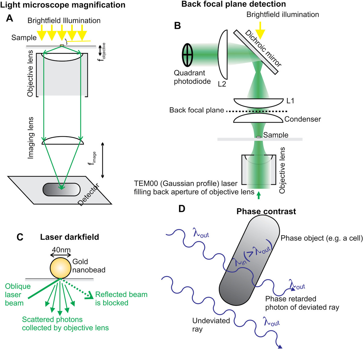
Figure 3.2 Light microscopy methods. (a) Magnification in the simplest two-lens light microscope. (b) Back focal plane detection (magnification onto quadrant photodiode is f2/f1 where fn is the corresponding focal length of lens Ln). (c) Laser dark field. (d) Phase retardation of light through a cell sample in phase contrast microscopy.
The two-lens microscope operates as a simple telescope system, with magnification M given by the ratio of the imaging lens focal length to that of the objective lens (the latter typically being a few millimeters):
(3.18)In practice, there are likely to be a series of several lens pairs placed between the imaging lens shown and the detector arranged in effect as telescopes, for example, with focal lengths f1, f2, f3, f4, …, fn corresponding to lenses placed between the objective lens and the camera detector. The magnification of such an arrangement is simply the multiplicative combination of the separate magnifications from each lens pair:
(3.19)Such additional lens pairs allow higher magnifications to be obtained without requiring a single imaging lens with an exceptionally high or low focal length, which would necessitate either an impractically large microscope or would result in severe optical aberration effects. A typical standard light microscope can generate effective total magnifications in the range 100–1000.
3.3.2 Depth of Field
The depth of field (df, also known as the “depth of focus”) is a measure of the thickness parallel to the optical axis of the microscope over which a sample appears to be in focus. It is conventionally defined as one quarter of the distance between the intensity minima parallel to the optic axis above and below the exact focal plane (i.e., where the sample in principle should be most sharply in focus) of the diffraction image that is produced by a single-point source light emitting object in the focal plane. This 3D diffraction image is a convolution of the point spread function (PSF) of the imaging system with a delta function. On this basis, df can be approximated as
(3.20)where
- λ is the wavelength of light being detected
- nm is the refractive index of the medium between the microscope objective lens or numerical aperture NA and the glass microscope coverslip/slide (either air, nm = 1, or for high-magnification objective lenses, immersion oil, nm = 1.515
- dR is the smallest length scale feature that can be resolved by the image detector (e.g., the pixel size of a camera detector) such that the image is projected onto the detector with a total lateral magnification of ML between it and the sample.
3.3.3 Light Capture from the Sample
The NA of an objective lens is defined nm sin θ, where nm is the refractive index of the imaging media. The angle θ is the maximum half-angle subtended ray of light scattered from the sample, which can be captured by the objective lens. In other words, higher NA lenses can capture more light from the sample. In air, nm = 1 so to increase the NA, further high-power objective lenses use immersion oil; a small blob of imaging oil is placed in optical contact between the glass microscope slide or coverslip and the objective lens, which has the same high value of refractive index as the glass.
The solid angle Ω subtended by this maximum half angle can be shown using simple integration over a sphere to be
(3.21)Most in vivo studies, that is, those done on living organisms or cells, are likely to be low magnification ML ~ 100 using a low numerical aperture objective lens of NA ~ 0.3 such as to encapsulate a large section of tissue on acquired images, giving a df of ~10 μm. Cellular studies often have a magnification an order of magnitude greater than this with NA values of up to ~1.5, giving a df of 0.2–0.4 μm.
Note that the human eye has a maximum numerical aperture of ~0.23 and can accommodate typical distances between ~25 cm and infinity. This means that a sample viewed directly via the eye through a microscope eyepiece unit, as opposed to imaged onto a planar camera detector, can be observed with a far greater depth of field than Equation 3.20 suggests. This can be useful in terms of visual inspection of a sample prior to data acquisition from a camera device.
3.3.4 Photon Detection at the Image Plane
The technology of photon detection in light microscopes has improved dramatically over the past few decades. Light microscopes use either an array of pixel detectors in a high-sensitivity camera, or a single detector in the form of a PMT or avalanche photodiode (APD). A PMT utilizes the photoelectric effect on a primary photocathode metal-based scintillator detector to generate a primary electron following absorption of an incident photon of light. This electrical signal is then amplified through secondary emission of electrons in the device. The electron multiplier consists of a series of up to 12 anodes (or dynodes) held at incrementally higher voltages, terminated by a final anode. At each anode/dynode, ~5 new secondary electrons are generated for each incident electron, indicating a total amplification of ~108. This is sufficient to generate a sharp current pulse, typically 1 ns, after the arrival of the incident photon, with a sensitivity of single-photon detection.
An APD is an alternative technology to a PMT. This uses the photoelectric effect but with semiconductor photon detection coupled to electron–hole avalanche multiplication of the signal. A high reverse voltage is applied to accelerate a primary electron produced following initial photon absorption in the semiconductor with sufficient energy to generate secondary electrons following impact with other regions of the semiconductor (similarly, with a highly energetic electron hole traveling in the opposite direction), ultimately generating an enormous amplification of free electron–hole pairs. This is analogous to the amplification stage in a PMT, but here the amplification occurs in the same semiconductor chip. The total multiplication of signal is >103, which is less sensitive than a PMT, however still capable of single-photon detection with an advantage of a much smaller footprint, permitting in some cases a 2D array of APDs to be made, similar to pixel-based camera detectors.
Many light microscopes utilize camera-based detection over PMT/APD detection primarily for advantages in sampling speed in not requiring slow mechanically scanning over the sample. Several standard light microcopy investigations that are not photon limited (e.g., bright-field investigations) use CCD image sensors, with the most sensitive light microscopes using electron-multiplying CCD (EMCCD) detection or complementary MOS (CMOS) technology. A CCD image sensor contains a 2D array composed of individual p-doped metal-oxide semiconductor (MOS) pixels. MOS pixels act as micron length scale capacitors with a voltage bias set just above the threshold for inversion, which thus generates electrons and holes on absorption of incoming photons.
Each MOS capacitor accumulates an electric charge proportional to the light absorbed, and control circuitry transfers this charge to its neighbor along each 1D line of the pixel, such that the last MOS capacitor in the line dumps its charge into the MOS pixel in the next line up or down, ultimately with all the charge transferred into an amplifier. This serial voltage data stream can then be subsequently reconstructed as a 2D image. A variant on the CCD includes the intensified CCD (ICCD) that comprises an initial detection step on a phosphor screen, with this phosphor light image then detect by a CCD behind it, which improves the ultimate photon detection efficiency to >90%.
Many cheaper cameras utilize a CMOS chip (these are now found ubiquitously in webcams, mobile phone cameras, and also in microprocessors in nonimaging applications). The core feature of a CMOS chip is a symmetrical back-to-back combination of n- and p-type MOS field effect transistors, requiring less additional circuitry with greater power efficiency compared to CCD pixels, manifest ultimately substantially faster imaging speeds. A scientific CMOS camera has an inferior photon collection efficiency of ~50% compared to ICCDs or EMCCDs, but can acquire data faster by an order of magnitude or more, equivalent to several thousand image frames per second.
An EMCCD utilizes a solid-state electron-multiplying step at the end of each line of CCD pixels. This amplifies relatively weak electrical signal above any readout noise that is added from the final output amplification step. This electron multiplication has normally a few hundred stages during which electrons are transferred by impact ionization, which generates multiple secondary electrons to amplify the signal. The resultant amplification is up to ~103, which compares favorably to APDs and ICCDs but with a much-reduced readout noise. EMCCDs are currently the photon detection tool of choice for low-light microscopy investigations in biology, having up to ~95% photon detection efficiency, for example, applied to single-molecule fluorescence detection, and have a reasonable sampling speed equivalent to ~1 ms per image frame for small pixel arrays of ~100 pixels of edge length, relevant to many fast biological processes.
3.4 Nonfluorescence Microscopy
Basic light microscopy is invaluable as a biophysical tool. However, its biggest weakness is poor image contrast, since most of the material in living organisms is water, on average ~60%. Since cells are surrounded by a fluid environment, which is largely water, the signal obtained from VIS light scattered from cellular object is small. However, there are several adaptations to basic light microscopy that can be applied to enhance image contrast.
3.4.1 Bright-Field and Dark-Field Microscopy
Bright-field microscopy relies on measuring the differences in the absorbed or scattered intensity of light as it passes through different features of the sample. Incident light is generated usually from either a tungsten halogen filament broadband source or a bright LED, which is captured by short focal length collector lens. Light is then directed through a condenser lens using a Köhler illumination design that involves forming an image of the light source in the back focal plane of the condenser (Figure 3.2b). This results in a collimated beam incident on the sample and a uniform illumination intensity in the focal plane of the microscope.
A cell on a microscope coverslip/slide whose shape is broadly symmetrical on either side of a plane parallel to a focal plane taken through its midheight will exhibit minimal bright-field image contrast between the foreground cellular material and the background cell media. A simple approach to increase the contrast for the outline of the cell is to use defocusing microscopy. Negative defocusing, for which the focal plane is moved below the midheight level of the cell closer to the object lens, generates an image of a dark cell body with a higher-intensity cell perimeter, while positive defocusing generates the inverse of this, due to light interference at the image plane between undeviated and transmitted light beams whose optical path length (OPL), which is the product of the geometrical path length of the light beam with the index of refraction in that optical media, depends upon the extent of defocus. The contrast at the cell perimeter is a function of the radius of curvature of the cell, and for cells of a micron length scale a defocus value of a few hundred nanometers generates optimum perimeter contrast.
Another approach to improve contrast is to tag a biomolecule with a reporter probe designed to generate a high local signal upon excitation with light, for example, a probe coated in a high atomic number metal such as gold generates a high scatter signal for certain wavelengths of VIS light. Here, photon scattering is elastic and so the wavelength of scattered light is the same as the incident light; thus, any scattered light not from the labeled biomolecules must be blocked. These include back reflections from the glass microscope coverslip/slide. The regions of the sample not containing tagged biomolecules appear dark on the camera detector, hence the name dark-field microscopy. In transmitted light dark field, a modified condenser lens blocks out the central aperture resulting in highly oblique illumination on the sample; nonscattered light will emerge at too steep an angle to be captured by the objective lens, whereas light diffracted by the sample will be forward scattered at small angles and can be captured.
A similar approach can be used with reflected light, in general using a laser source (hence laser dark field) in which an oblique angled laser beam incident on the sample emerging from the objective lens is either transmitted through the coverslip in the absence of any sample, or back scattered by the sample back into the objective lens (Figure 3.2c). An additional enhancement of contrast can be achieved by the generation of surface plasmons, whose intensity is a function of the particle size (a few tens of nanometers) and the laser wavelength. This can generate very high SNRs on in vitro samples facilitating extremely high time resolutions of ~10−6 s.
Dark-field microscopy has more limited use with living samples than bright-field microscopy because the relatively large size of a cell compared to the scatter signal either from a native unlabeled biomolecule or from a biomolecule that has been labeled using a dark-field probe (e.g., a gold-coated bead of tens of nanometers in diameter) can result in significant scatter from the cell body itself, which can swamp the probe signal. The scatter signal from unlabeled biomolecules can be prohibitively small, but using a scatter label can also present technical challenges; it is not easy to specifically label biomolecules inside living cells with, for example, a gold nanoscale bead without nonspecific labeling of other cellular structures.
For certain cell types (e.g., prokaryotes), it is also difficult to introduce such a large scatter probe while still keeping the cell intact, limiting its application to accessible surface features. The practical lower size limit to detect a reproducible, measurable signal from the scattered light is a few tens of nanometers; the size of the probe is large compared to single biomolecules implying some steric hindrance effects with impairment of normal biological operation. Note that there are advanced new techniques such as interferometric scattering microscopy, which use interferometric methods of scattered light detection that can be used to detect the scattered signal directly from unlabeled biomolecules themselves (see Chapter 4).
3.4.2 Contrast Enhancement Using Optical Interference
Optical interference techniques can be used to modify a light microscope to increase image contrast. Phase contrast microscopy utilizes differences in refractive index inside a biological sample. Optically, transparent cells and tissues exhibit a range of refractive indices nt as a function of spatial localization across the tissue, 1.35–1.45 being typical for cellular material, which compares with that of water, nw ~ 1.33. The result is that the phase of light propagating through a region of sample, which has a length parallel to the optic axis Δz of a few microns, will be retarded. Such objects are examples of phase objects. The retardation for many cells is roughly around a quarter of a wavelength λ relative to that of light passing through the largely aqueous environment in between cells (Figure 3.2d). It is trivial to derive the following relationship by comparing the speed of light in water to that inside a cell or tissue on the basis of differences in refractive indices:
(3.22)An annulus aperture in the front focal plane of the condenser lens, similar to that used for dark-field forward scatter microscopy in blocking out the central aperture of illumination, generates a cone of collimated light onto the sample. Emergent light transmitted through the sample is collected by an objective lens consisting of both undeviated light (since the angle of the cone of light is not as oblique as that used in dark-field microscopy) that has not encountered any biological material and diffracted (forwarded scattered) light that has exhibited a relative phase retardation to the undeviated light.
A phase ring in the back focal plane of the objective lens, in a conjugate image plane to the condenser annulus, converts this retardation into a half wavelength phase shift, a condition for destructive interference, either by introducing a half wavelength phase increase in the ring (positive phase contrast microscopy) by having an extra thickness of glass, for example, in which case the background appears darker relative to the foreground sample, or more commonly by introducing a further half wavelength phase retardation in the ring (negative phase contrast microscopy) by indenting the glass in that region, in which case the sample appears brighter relative to the background, or by coating the ring in a thin layer of aluminum.
In other words, this process transforms phase information at the sample into amplitude contrast in the intensity of the final image. The length scale of a few microns over which the retardation of the light is typically a quarter of a wavelength is comparable to some small cells in tissues, as well as cellular organelle features such as the nucleus and mitochondria. It is therefore ideal for enhancing the image contrast of cellular components.
Polarized light microscopy can increase the relative contrast of birefringent samples. Birefringence, as discussed for polarization spectroscopy techniques in Section 3.2.4, occurs when a sample has a refractive index which is dependent upon the orientation of the polarization E-field vector of the incident light. This is often due to repeating structural features in a sample, which have a spatial periodicity over a length scale comparable to, or less than, the wavelength of the light, which is true for several biological structures. In other words, this is a characteristic of certain crystals or more relevant for biological samples due to the fluidity of the water-solvent environment and other fluidic structures such as phospholipid bilayers, liquid crystals.
There are several examples of birefringent biological liquid crystals. These include fibrous proteins with well-defined spatial periodicity between bundles of smaller fibrils such as collagen in the extracellular matrix, cell membranes and certain proteins in the cell membranes, cytoskeletal proteins, structural proteins in the cell walls of plants (e.g., cellulose) and certain bacteria (e.g., proteoglycans), and the highly periodic protein capsid coats of viruses. Polarization microscopy is an excellent tool for generating images of these biological liquid crystal features, and there are also examples of nonliquid crystalline biomolecule samples that can be investigated similarly (e.g., crystalline arrays of certain vitamins).
For polarization microscopy, a polarizer is positioned in the illumination path between the VIS light source and a condenser lens, before the sample, and a second polarizer described as an analyzer is positioned after the transmitted light has emerged from the sample, close to the back aperture of the objective lens. The transmitted light through a birefringent sample can be split into two orthogonally polarized light components of p and s, which are either parallel to the plane of the optic axis or perpendicular to it, respectively. The speed of the light in each of these separate components is different due to the polarization dependence of the refractive index in the sample. These components therefore become out of phase with each other but are recombined with various combinations of constructive and destructive interference during their passage through the analyzer, depending upon the relative position on the sample, which is then imaged onto a camera (or viewed through eyepieces) in the normal way for basic light microscopy. Polarized light microscopy can quantify the precise amount of retardation that occurs in each polarization direction and thus generates information about the relative orientation of spatially periodic molecular structures of the birefringent sample. Some of these structures are involved in mechanical features of tissues and cells, and thus polarization microscopy can be used to probe biomechanics (see Chapter 6).
Differential interference contrast (DIC) microscopy is a related technique to polarization microscopy, in using a similar interference method utilizing polarized light illumination on the sample. A polarizer again is placed between the VIS light source and condenser lens, which is set at 45° relative to the optical axis of an additional birefringent optical component of either a Wollaston prism or a Nomarski compound prism, which is positioned in the beam path in the front focal plane of the condenser lens. These prisms both generate two transmitted orthogonally polarized rays of light, referred to as the “ordinary ray” (polarized parallel to the prism optical axis) and the “extraordinary ray,” thus with polarization E-field vectors at 0°/90° relative to the prism optic axis. These two rays emerge at different angles relative to the incident light (which is thus said to be sheared), their relative angular separation called the “shear angle,” due to their different respective speeds of propagation through the prism (Figure 3.3a).
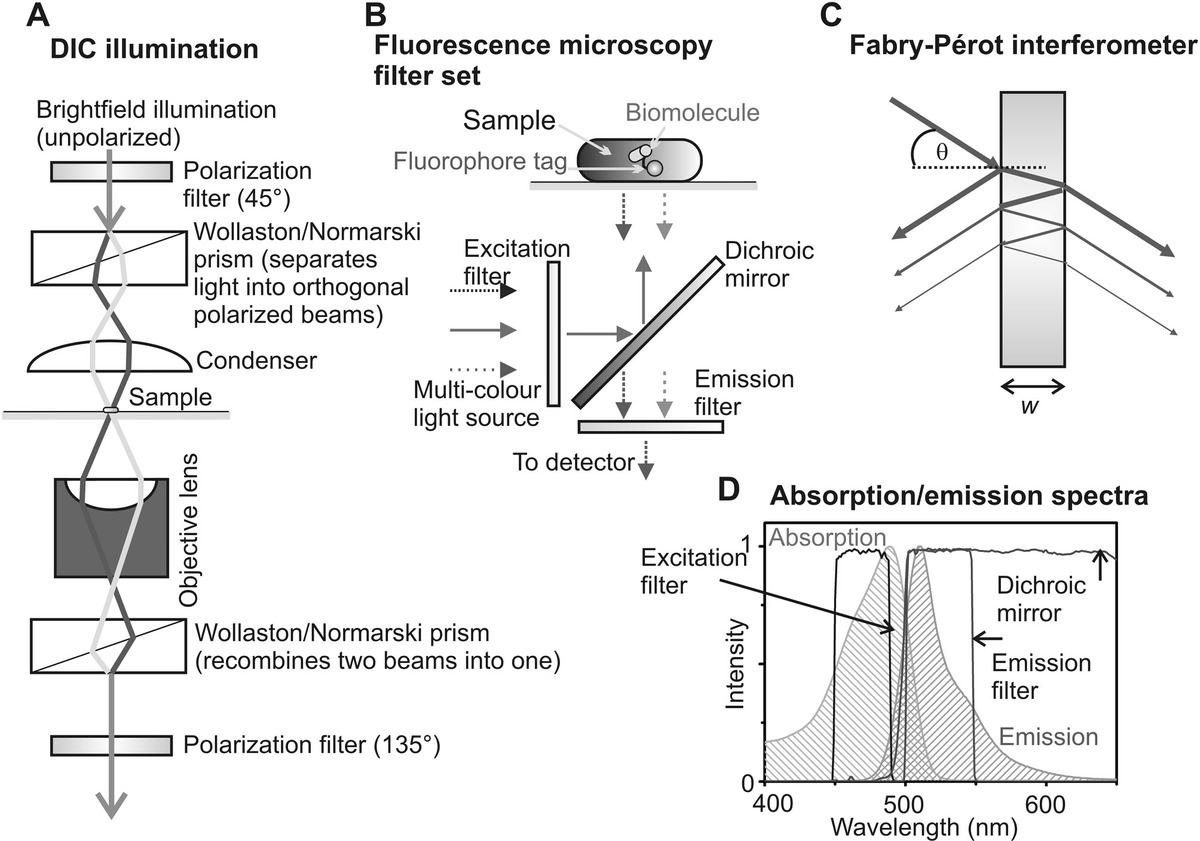
Figure 3.3 Generating image contrast in light microscopy. (a) Schematic of differential interference contrast illumination. (b) Typical fluorescence microscopy filter set. (c) Wavelength selection using a Fabry–Perot interferometer design. (d) Absorption and emission spectra for GFP, with overlaid excitation and emission filters and dichroic mirror in GFP filter set.
These sheared rays are used to form a separate sample ray and reference ray, which are both then transmitted through the sample. After passing through the sample and objective lens, both transmitted sheared rays are recombined by a second matched Wollaston/Nomarski prism positioned in a conjugate image plane to the first, with the recombined beam then transmitted through a second polarizer analyzer oriented to transmit light polarized at 135°. The difference in OPLs of the sample and reference beam results in an interference pattern at the image plane (normally a camera detector), and it is this wave interference that creates contrast.
Since the sample and reference beams emerge at different angles from the first Wollaston/Nomarski prism, they generate two bright-field images of orthogonal polarization that are laterally displaced from each other by typically a few hundred nanometers, with corresponding regions of the two images resulting from different OPLs, or phases. Thus, the resultant interference pattern depends on the variations of phase between lateral displacements of the sample, in other words with the spatial gradient of refractive index of across a biological sample. It is therefore an excellent technique for identifying the boundaries of cells and also of cell organelles.
A related technique to DIC using polarized illumination is Hoffmann modulation contrast (HMC) microscopy. HMC systems consist of a condenser and objective lens, which have a slit aperture and two coupled polarizers instead of the first Wollaston/Nomarski prism and polarizer of DIC, and a modulator filter in place of the second Wollaston/Nomarski prism, which has a spatial dependence on the attenuation of transmitted light. This modulator filter has usually three distinct regions of different attenuation, with typical transmittance values of T = 100% (light), 15% (gray), and 1% (dark). The condenser slit is imaged onto the gray zone of the modulator. In regions of the sample where there is a rapid spatial change of sample optical path, refraction occurs, which deviates the transmitted light path. The refracted light will be attenuated either more or less in passing through the modulator filter, resulting in an image whose intensity values are dependent on the spatial gradient of the refractive index of the sample, similar to DIC. HMC has an advantage over DIC in that it can be used with birefringent specimens, which would otherwise result in confusing images in DIC, but has a disadvantage in that DIC can utilize the whole aperture of the condenser resulting in higher spatial resolution information from the transmitted light.
Quantitative phase imaging (QPI) (Popescu, 2011) utilizes the same core physics principles as phase microscopy but renders a quantitative image in which each pixel intensity is a measure of the absolute phase difference between the scattered light from a sample relative to a reference laser beam and has the same advantages of being label-free and thus less prone to potential physiological artifacts due to the presence of a contrast-enhancing label such as a fluorescent dye. It can thus in effect create a map of the variation of the refraction index across a sample, which is a proxy for local biomolecular concentration—for example, as a metric for the spatial variation of biomolecular concentration across a tissue or in a single cell. 2D and 3D imaging modalities exist, with the latter also referred to as holotomograpy. The main drawback of QPI is the lack of specificity since it is non-trivial to deconvolve the respective contributions of different cellular biomolecules to the measured refractive index. To mitigate this issue, QPI can be also combined with other forms of microscopy such as fluorescence microscopy in which specific fluorescent dye labeling can be used with multicolor microscopy to map out the spatial distribution of several different components (see section 3.5.3), while QPI can be used to generate a correlated image of the total biomolecular concentration in the same region of the cell or tissue sample. Similarly, QPI can be correlated with several other light microscopy techniques, for example including optical tweezers (see Chapter 6).
3.4.3 Digital Holographic Microscopy
Digital holographic microscopy is emerging as a valuable tool for obtaining 3D spatial information for the localization of swimming cells, for example, growing cultures of bacteria, as well as rendering time-resolved data for changes to cellular structures involved in cell motility during their normal modes of action, for example, flagella of bacteria that rotate to enable cells to swim by using a propeller type action, and similarly cilia structures of certain eukaryotic cells. The basic physics of hologram formation involves an interference pattern between a laser beam, which passes through (or some variant of the technique is reflected from) the sample, and a reference beam split from the same coherent source that does not pass through the sample. The sample beam experiences phase changes due to the different range of refractive indices inside a cell compared to the culture medium outside the cell, similar to phase contrast microscopy. The interference pattern formed is a Fourier transform of the 3D variation of relative phase changes in the sample and therefore the inverse Fourier transform can render 3D cellular localization information.
Several bespoke digital holographic systems have been developed for studying dense cultures of swimming cells in particular to permit the investigation of biological physics features such as hydro-dynamic coupling effects between cells as well as more physical biology effects such as signaling features of swimming including bacterial chemotaxis, which is the method by which bacteria use a biased random walk to swim toward a source of nutrients and away from potential toxins. Some systems do not require laser illumination but can function using a relatively cheap LED light source, though they require in general an expensive camera that can sample at several thousand image frames per second in order to obtain the time-resolved information required for fast swimming cells and rapid structural transitions of flagella or cilia.
3.5 Fluorescence Microscopy: The Basics
Fluorescence microscopy is an invaluable biophysical tool for probing biological processes in vitro, in live cells, and in cellular populations such as tissues. Although there may be potential issues of phototoxicity as well as impairment of biological processes due to the size of fluorescent “reporter” tags, fluorescence microscopy is the biophysical tool of choice for investigating native cellular phenomena in particular, since it provides exceptional detection contrast for relatively minimal physiological perturbation compared to other biophysical techniques. It is no surprise that the number of biophysical techniques discussed in this book is biased toward fluorescence microscopy.
3.5.1 Excitation Sources
The power of the excitation light from either a broadband or narrow bandwidth source may first require attenuation to avoid prohibitive photobleaching, and related photodamage, of the sample. Neutral density (ND) filters are often used to achieve this. These can be either absorptive or reflective in design, which attenuate uniformly across the VIS light spectrum, with the attenuation power of 10ND where ND is the neutral density value of the filter. Broadband sources, emitting across the VIS light spectrum, commonly include the mercury arc lamp, xenon arc lamp, and metal–halide lamp. These are all used in conjunction with narrow bandwidth excitation filters (typically 10–20 nm bandwidth spectral window), which select specific regions of the light source spectrum to match the absorption peak of particular fluorophores to be used in a given sample.
Narrow bandwidth sources include laser excitation, with an emission bandwidth of around a nanometer. Bright LEDs can be used as intermediate bandwidth fluorescence excitation source (~20–30 nm spectral width). Broadband lasers, the so-called white-light supercontinuum lasers, are becoming increasingly common as fluorescence excitation sources in research laboratories due to reductions in cost coupled with improvements in power output across the VIS light spectrum. These require either spectral excitation filters to select different colors or a more dynamic method of color selection such as an acousto-optic tunable filter (AOTF).
The physics of AOTFs is similar to those of the acousto-optic deflector (AOD) used, for example, in many optical tweezers (OT) devices to position laser traps and are discussed in Chapter 5. Suffice to say here that an AOTF is an optically transparent crystal in which a standing wave can be generated by the application of radio frequency oscillations across the crystal surface. These periodic features generate a predictable steady-state spatial variation of refractive index in the crystal, which can act in effect as a diffraction grating. The diffraction angle is a function of light’s wavelength; therefore, different colors are spatially split.
The maximum switching frequency for an AOTF (i.e., to switch between an “off” state in which the incident light is not deviated, and an “on” state in which it is deviated) is several tens of MHz; thus, an AOTF can select different colors dynamically, more than four orders of magnitude faster than the sampling time of a typical fluorescence imaging experiment, though the principal issues with an AOTF is a drop in output power of >30% in passing through the device and the often prohibitive cost of the device.
3.5.2 Fluorescence Emission
The difference in wavelength between absorbed and emitted light is called the Stokes shift. The full spectral emission profile of a particular fluorophore, φEM(λ), is the relation between the intensity of fluorescence emission as a function of emission wavelength normalized such that the integrated area under the curve is 1. Similarly the spectral excitation profile of a particular fluorophore, φEX(λ), represents the variation of excitation absorption as a function of incident wavelength, which looks similar to a mirror image of the φEM(λ) profile offset by the Stokes shift.
A typical fluorescence microscope will utilize the Stokes shift by using a specially coated filter called a dichroic mirror, usually positioned near the back aperture of the objective lens in a filter set consisting of a dichroic mirror, an emission filter, and, if appropriate, an excitation filter (Figure 3.3b). The dichroic mirror reflects incident excitation light but transmits higher wavelength light, such as that from fluorescence emissions from the sample. All samples also generate elastically scattered light, whose wavelength is identical to the incident light. The largest source of elastic back scatter is usually from the interface between the glass coverslip/slide on which the sample is positioned and the water-based solution of the tissue often resulting in up to ~4% of the incident excitation light being scattered back from this interface. Typical fluorescent samples have a ratio of emitted fluorescence intensity to total back scattered excitation light of 10−4 to 10−6. Therefore, the dichroic mirror ideally transmits less than a millionth of the incident wavelength light.
Most modern dichroic mirrors operate as interference filters by using multiple etalon layers of thin films of dielectric or metal of different refractive indices to generate spectral selectivity in reflectance and transmission. A single etalon consists of a thin, optically transparent, refractive medium, whose thickness w is less than the wavelength of light, which therefore results in interference between the transmitted and reflected beams from each optical surface (a Fabry–Pérot interferometer operates using similar principles). With reference to Figure 3.3c, the phase difference Δφ between a pair of successive transmitted beams is
(3.23)where
- λ is the free-space wavelength
- n is the refractive index of the etalon material
The finesse coefficient F is often used to characterize the spectral selectivity of an etalon, defined as
(3.24)where R is the reflectance, which is also given by 1 – T where T is the transmittance, assuming no absorption losses. By rearrangement
(3.25)A maximum T of 1 occurs when the OPL difference between successive transmitted beams, 2nw cos θ, is an integer number of wavelengths; similarly the maximum R occurs when the OPL equals half integer multiples of wavelength. The peaks in T are separated by a width Δλ known as the free spectral range. Using Equations 3.23 through 3.25, Δλ is approximated as
(3.26)where λpeak is the wavelength of the central T peak. The sharpness of each peak in T is measured by the full width at half maximum, δλ, which can be approximated as
(3.27)Typical dichroic mirrors may have three or four different thin film layers that are generated by either evaporation or sputtering methods in a vacuum (see Chapter 7) and are optimized to work at θ = 45°, the usual orientation in a fluorescence microscope.
The transmission function of a typical VIS light dichroic mirror, TD(λ) is thus typically <10−6 for λ < (λcut-off − Δλcut-off/2) and more likely 0.90–0.99 for λ > (λcut-off + Δλcut-off/2), up until using the VIS light maximum wavelength of ~750 nm, where λcut-off is the characteristic cutoff wavelength between lower wavelength high attenuation and higher wavelength high transmission, which is usually optimized against the emission spectra of a particular fluorescent dye in question. The value Δλcut-off is a measurement of the sharpness of this transition in going from very high to very low attenuation of the light, typically ~10 nm.
In practice, an additional fluorescence emission filter is applied to transmitted light, bandpass filters such that their transmission function TEM(λ) is <10−8 for λ < (λmidpoint – Δλmidpoint/2) and for λ > (λmidpoint + Δλmidpoint/2) and for λ between these boundaries is more likely 0.90–0.99, where λmidpoint is the midpoint wavelength of the band-pass window and Δλmidpoint is the bandwidth of the window, ~10–50 nm depending on the fluorophore and imaging application (Figure 3.3d).
The fluorescence quantum yield (Φ) gives a measure of the efficiency of the fluorescence process as the ratio of emitted photons to photons absorbed, given by
(3.28)where
- ks is the spontaneous rate of radiative emission
- Φi and ki are the individual efficiencies and rates, respectively, for the various decay processes of the excited state (internal conversion, intersystem crossing, phosphorescence)
The fluorescence emission intensity IEM from a given fluorophore emitting isotropically (i.e., with equal probability in all directions), which is detected by a camera, can be calculated as
(3.29)where
- Iabs is the total absorbed light power integrated over all wavelengths
- Ω is the collection angle for photons of the objective lens
- TOTHER is a combination of all of the other transmission spectra of the other optical components on the emission path of the microscope
- Ecamera is the efficiency of photon detection of the camera
The total SNR for fluorescence emission detection is then
(3.30)where NEM is the number of detected fluorescence emission photons per pixel, with their summation being over the extent of a fluorophore image consisting of n pixels in total (i.e., after several capture and transmission losses, through the microscope) from a camera whose gain is G (i.e., for every photon detected the number of electron counts generated per pixel will be G) and readout noise per pixel is NCAM, with NEX photons transmitted over an equivalent region of the camera over which the fluorophore is detected.
3.5.3 Multicolor Fluorescence Microscopy
A useful extension of using a single type of fluorophore for fluorescence microscopy is to use two or more different fluorophore types that are excited by, and which emit, different characteristic ranges of wavelength. If each different type of fluorophore can be tagged onto a different type of biomolecule in an organism, then it is possible to monitor the effects of interaction between these different molecular components and to see where each is expressed in the organism at what characteristic stages in the lifecycle and how different effects from the external environment influence the spatial distributions of the different molecular components. To achieve this requires splitting the fluorescence emission signal from each different type of fluorophore onto a separate detector channel.
The simplest way to achieve this is to mechanically switch between different fluorescence filter sets catered for the different respective fluorophore types and acquire different images using the same region of sample. One disadvantage with this is that the mechanical switching of filter sets can judder the sample, and this coupled to the different filter set components being very slightly out alignment with each other can make it more of a challenge to correctly coalign the different color channel images with high accuracy, necessitating acquiring separate bright-field images of the sample for each different filter set to facilitate correct alignment (see Chapter 8).
A more challenging issue is that there is a time delay between mechanically switching filter sets, at least around a second, which sets an upper limit on the biological dynamics that can be explored using multiple fluorophore types. One way round this problem is to use a specialized multiple band-pass dichroic mirror in the filter set, which permits excitation and transmission of multiple fluorophore types, and then using one more additional standard dichroic mirrors and single band-pass emission filters downstream from the filter set to then split the mixed color fluorescence signal, steering each different color channel to a different camera, or onto different regions of the same camera pixel array (Figure 3.4a). Dual and sometimes triple-band dichroic mirrors are often used. The main issue with having more bands is that since the emission spectrum of a typical fluorophore is often broad, each additional color band results in losing some photons to avoid cross talk between different bands by bleed-through of the fluorescence signal from one fluorophore type into the detection channel of another fluorophore type. Having sufficient brightness in all color channels sets a practical limit on the number of channels permitted, though quantum dots (QDs) have much sharper emission spectra compared to other types of fluorophores and investigations can be performed potentially using up to seven detection bands across the VIS and near IR light spectrum.
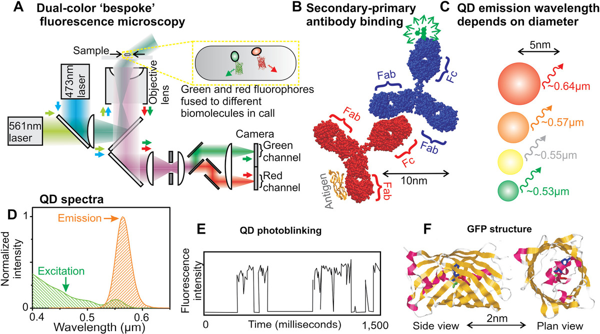
Figure 3.4 Fluorophores in biophysics. (a) Bespoke (i.e., homebuilt) dual-color fluorescence microscope used in imaging two fluorophores of different color in a live cell simultaneously. (b) Fluorescently labeled secondary antibody binding to a specific primary antibody. (c) Dependence of QD fluorescence emission wavelength on diameter. (d) Normalized excitation (green) and emission (orange) spectra for a typical QD (peak emission 0.57 μm). (e) Example fluorescence intensity time trace for a QD exhibiting stochastic photoblinking. (f) Structure of GFP showing beta strands (yellow), alpha helices (magenta), and random coil regions (gray).
3.5.4 Photobleaching of Fluorophores
Single-photon excitation of a bulk population of photoactive fluorophores of concentration C(t) at time t after the start of the photon absorption process follows the first-order bleaching kinetics, which is trivial to demonstrate and results in
(3.31)where tb is a characteristic photobleach time, equivalent to the lifetime of the fluorescence excited state. This photobleach time is the sum of an equivalent radiative decay time, trad (processes involving direct emission of photon radiation) and nonradiative decay time, tnon-rad (processes not involving the direct emission of photon radiation, such as molecular orbital resonance effects). In general, if there are a total of n fluorescence decay mechanisms, then
(3.32)where ki is the rate constant of the ith fluorescence decay mechanism. Photobleaching of each single fluorophore molecule is a stochastic Poisson process such that its photoactive lifetime is an exponential distribution of mean time tb. The principal cause of irreversible photobleaching of a fluorophore is light-dependent free radical formation in the surrounding water solvent, especially from molecular oxygen (under normal conditions, the concentration of dissolved oxygen in biological media is relatively high at ~0.5 mM, unless efforts are made to remove it). Free radicals are highly reactive chemicals containing an unpaired electron, which can combine with a fluorophore to destroy its ability to fluoresce. Many fluorophores also exhibit reversible photobleaching (or blinking), often under conditions of high excitation intensity, in which the excited state is transiently quenched to generate a stochastic dark “off” state as well as the bright “on” state.
Blinking is also known as fluorescence intermittency and is related to the competition between radiative and nonradiative relaxation pathways for the excited electron state (i.e., an excited state electron can return to its ground state via more than just a single energy transition pathway). The blinking phenomenon is exhibited by many fluorophores, especially semiconductor-based systems such as quantum dots, and also organic dyes and fluorescent proteins (FPs) (see the following sections in this chapter). Blinking often appears to obey a power-law distribution of on and off times with dark states in some systems lasting for tens of seconds, which is enormous on the quantum time scale, but remarkably a dark blinker will recover its fluorescence state after such a huge dark period and start emitting once again. The underlying specific physical mechanisms for blinking are largely unresolved but appear to be very specific for the fluorophore type.
3.5.5 Organic Dye Fluorophores
There are a large range of different organic dyes, for example, cyanines and xanthenes, whose chemical structures facilitate electron delocalization through a so-called π-electron system. A π bond is a covalent molecular orbital formed from the overlap of two p atomic orbitals; multiple π bonds in close proximity in a molecular structure can form a pool of spatially extended, delocalized electron density over a portion of the molecule through orbital resonance. This enables a large portion of the molecule to operate as an efficient electric dipole.
Historically, such dyes were first used to specifically label single biomolecules using immunofluorescence. Here, a primary antibody binds with high specificity to the biomolecule of interest, while a secondary antibody, which is chemically labeled with one or more fluorophores, then binds to the primary antibody (Figure 3.4b). The main issues with this technique concern the size of the probe and how to deliver it into a cell. The effective size of the whole reporter probe is ~20 nm, since each antibody has an effective viscous drag radius (the Stokes radius) of ~10 nm, which is an order of magnitude larger than some of the biomolecules being labeled. This can impair their biological functions. Second, introducing the antibody labels into living tissue is often difficult without significantly impairing the physiological functions, for example, permeabilizing the tissue using harsh detergents. With this caveat, this can result in very informative fluorescence images in vivo.
Fluorescence in situ hybridization (FISH) is a valuable labeling technique using organic dyes for probing specific regions of nucleic acids. A probe consists of a ~10 nucleotide base sequence either of singled-stranded DNA or RNA, which binds to a specific sequence of nucleic acid from a cell extract or a thin, fixed (i.e., dead) tissue sample via complementary base pairing following suitable incubation protocols normally >10 h, sometimes a few days. A fluorophore either is chemically attached to the FISH probe via one or more bases via a fluorescent secondary antibody or is a chemical tag that binds to the probe. FISH can isolate the position of individual genes and can be used clinically in probing a range of disorders in a developing fetus in the womb by testing extracts of amniotic fluid.
Fluorophores can also use covalent chemical conjugation to attach to specific biological molecules. For example, a common strategy is to use the reactive sulfhydryl (–SH) side group of cysteine amino acids in proteins to conjugate to a fluorophore a dye molecule to generate a new thiol covalent bond (–S–R where R is the chemical group of the dye molecule). Proteins that contain several cysteine amino acid groups can lead to problems due to multiple labeling, and genetic modifications are often performed to knock out some of these additional cysteine residues. In addition, proteins that contain no native cysteines can be genetically modified to introduce an additional foreign cysteine. This general technique is called “site-specific cysteine mutagenesis.”
Other less specific chemical conjugation methods exist. These methods target more general reactive chemical groups, including amino (–NH2) and carboxyl (–COOH) groups, especially those present in the substituent group of amino acids. The principal issue is that the binding target is not specific and so dye molecules can bind to several different parts of a biomolecule, which makes interpretation of imaging data more challenging, in addition to potentially affecting biological function of the molecule in unpredictable ways. Click chemistry is an alternative method of conjugation. The “click” is meant to convey a convenience of simply snapping objects together. The most utilized type of click chemistry relies on strong covalent bonds formed between a reacting azide and a carbon–carbon alkyne triple bond. The main challenge is to introduce the foreign chemical group, either the azide or alkyne, into the biomolecule. With DNA, a variety of foreign chemical conjugating groups can be introduced using oligo inserts. These are short ~10 bp sections of DNA whose sequence is designed to insert at specific regions of the large DNA molecule used under in vitro investigation, and each oligo insert can be manufactured to be bound to a specific chemical group for conjugation (e.g., azide and biotin). All chemical conjugation techniques are discussed in more detail in Chapter 7.
Organic dye fluorophores may also be conjugated to small latex beads that have a typical diameter of a few hundred nanometers, small microspheres or large nanospheres depending on which way you look at it, which may then be conjugated to a biological substructure to yield a brighter probe that permits faster imaging. The biggest disadvantage is the size of these sphere probes, which is large enough to impair the normal biological processes in some way.
Most organic dye fluorophores emit VIS light. However, VIS light results in greater elastic scattering from unlabeled surrounding tissue, manifested as noise in fluorescence microscopy. Progress in developing fluorophores that are excited at longer wavelengths, some even in the IR region, is of assistance here.
3.5.6 FlAsH/ReAsH Probes
Improvements in minimizing biological process impairments are offered through the use of the green fluorescein arsenical helix (FlAsH) binder and the pink organic dye resorufin (ReAsH). This technology utilizes a genetically encoded arrangement of four cysteine amino acid residues in a specific protein under study inside a cell. Cells are incubated with membrane-permeable FlAsH/ReAsH reagents, which can then bind to the four cysteine residues inside the cell, which convert the dyes into a fluorescent form. FlAsH/ReAsH reagents have an effective diameter of 1–2 nm with a binding site in a protein requiring as few as six amino acids (four for the cysteine residues plus two more to generate the 3D shape for a binding pocket) and therefore exhibit minimal steric hindrance effects. But it is technically difficult to introduce the reagents, and the nonspecificity of binding combined with cellular toxicity has limited its use.
3.5.7 Semiconductors, Metal-Based Fluorophores, and Nanodiamonds
Other fluorescent probes that have been applied to populations of cells include semiconductor-based fluorescent nanocrystals that generate quantized excitation energy states that relate not only to the material properties of their crystals but also to their physical dimensions and shapes. These include primarily quantum rods and QDs. The physics of their fluorescence properties are similar, and we use QDs as an exemplar here since these, in particular, have found significant applications in biophysics. They have advantages of being relatively bright, but their diameter is roughly an order of magnitude smaller than micro-/nanospheres. QDs have a photostability >100 times that of most organic dyes and so can be considered not to undergo significant irreversible photobleaching for most experimental applications. They thus have many advantages for monitoring single biomolecules. They are made from nanocrystal alloy spheres typically of two to three components (cadmium selenide (CdSe) and cadmium telluride (CdTe) are the most common) containing ~100 atoms. They are ~3–5 nm in core diameter (Figure 3.4c) and have semiconductor properties, which can undergo fluorescence due to an exciton resonance effect within the whole nanocrystal, with the energy of fluorescence relating to their precise length scale dimensions. An exciton is a correlated particle pairing composed of an electron and electron hole. It is analogous to the excited electron state of traditional fluorophores but has a significantly longer lifetime of ~10−6 s.
The fluorescence emission spectrum of a QD is dependent on its size. A QD is an example of quantum confinement of a particle in a box in all three spatial dimensions, where the particle in question is an exciton. In other words, QDs have size-dependent optical properties. The 1D case of a particle in a box can be solved as follows. The Schrödinger equation can be written as
(3.33)where
- ψ(x) is the wave function of a particle of mass m at distance x
- V is the potential energy
- E is the total energy
- h is Planck’s constant
For a “free” particle, V is zero, and it is trivial to show that a sinusoidal solution exists, such that if the probability of being at the ends of the “1D box” (i.e., a line) of length a is zero, this leads to allowed energies of the form
(3.34)where n is a positive integer (1, 2, 3, …); hence, the energy levels of the particle are discrete or quantized. This formulation can be generalized to a 3D Cartesian box of dimensions a, b, and c parallel to the x, y, and z axes, respectively, which yields solutions of the form
(3.35)QDs, however, has a spherical geometry, and so Schrödinger’s equation must be solved in spherical polar coordinates. Also, the different effective masses of the electron me and hole mH (mH > me in general) need to be considered as do the electrostatic ground state energy and the bulk energy of the semiconductor, which leads to
(3.36)where
- q is the unitary electron charge
- Ebulk is the bulk semiconductor energy
- εr and ε0 are the relative electrical permittivity and absolute electrical permittivity in a vacuum
- a is the QD radius
When light interacts with a QD, an electron–hole exciton pair is created. An exciton has an associated length scale called the Bohr radius, such that beyond this length scale, the probability of exciton occurrence is very low. For CdSe QDs, the Bohr radius is ~5.6 nm, and thus quantum confinement effects occur at QD diameters that are less than ~11.2 nm. The aforementioned equation predicts that the energy state of the confined exciton decreases with increasing QD radius. In other words, smaller QDs are blue, while larger QDs are red.
QDs are characterized by a broad absorption spectrum and narrow emission spectrum—this means that they can be excited using a range of different lasers whose wavelength of emission does not necessarily correspond to an absorption peak in the fluorophore as is the case for organic dyes, with the tightness of the spectral emission meaning that emissions can be relatively easily filtered without incurring significant loss of signal (Figure 3.4d).
This narrowness of spectral emission means that several different colored QDs can be discriminated in the same sample on the basis of their spectral emission, which is useful if each different colored QD tags a different biomolecule of interest. QDs are brighter than their corresponding organic dyes at similar peak emission wavelength; however, their relative brightness is often overstated (e.g., a single QD emitting in the orange-red region of the VIS light spectrum at the corresponding excitation wavelengths and powers is typically only six to seven times brighter than a single molecule of the organic dye rhodamine).
QDs undergo a photophysical phenomenon of blinking (Figure 3.4e). Many different types of fluorophores also undergo blinking. Blinking is a reversible transition between a photoactive (light) and an inactive (dark) state; the dye appears to be bright and then momentarily dark in a stochastic manner (i.e., random with respect to time), but, in general, these are prevalent more at excitation intensities higher than would normally be used for fluorescence imaging with dark state dwell times <10 ms, which is often sufficiently fast to be averaged out during typical fluorescence microscopy sampling time windows of ~100 ms or more. QDs blink more appreciably at lower excitation intensities with longer dwell times of dark states more comparable to the time scale of typical fluorescence imaging, which can make it difficult to assess if what you see from one image to a consecutive image in a kinetic series of images is a continuous acquisition of the same tagged biomolecule or a different one that has diffused in to the field of view from elsewhere.
The actual functional diameter of a QD can be more like 15–20 nm since the core is further coated with a solvent-protective shell (typically zinc sulfide) and a polymer matrix for chemical functionalization. The size can increase further to ~30 nm if an antibody is also attached to the QD to allow more specific binding to a given biological molecule. A diameter of 30 nm is an order of magnitude larger than a typical biomolecule, which can result in significant steric hindrance effects, which can inhibit native biological processes and also make it challenging to deliver the QD into a cell. However, there have been several applications of cellular imaging developed using QD fluorophores, going back to the turn of the century (see Michalet et al., 2005).
An alternative metal-based fluorophore involves lanthanides. The lanthanides are a group of 15 4f-orbital metals in the periodic table between atomic number element 57 (lanthanum) to 71 (lutetium). They form unique fluorescent complexes when bound via their 3+ ion states with an organic chelating agent, such as a short random coil sequence of a given protein to be labeled. This can confer significant stability to the fluorophore state, since the chelation complex is protected from water and so exhibits limited free radical photobleach damage (Allen and Imperiali, 2010).
Fluorescent nanodiamond (FND) is emerging as a valuable probe for biological samples since it has a high photostability manifest as no photobleaching or blinking, is biocompatible, and has spectral properties that are relatively insensitive to the surrounding fluid environment and are spectrally distinct from the normal range of cellular autofluorescence. A nanodiamond is a synthetic nanoscale-sized particle composed of carbon atoms bound in the tetrahedral sp3 arrangement (see Chapter 2), identical to that of natural diamond. The fluorescence comes from doping the center of the nanodiamond with a high density of negatively charged nitrogen vacancy (NV–) atoms. NV– is a fluorophore with peak absorption wavelength of roughly 550 nm, emitting at ~700 nm, and so not only has a wide Stokes shift facilitating fluorescence detection, but also emits at wavelengths which are 200–300 nm higher than typical contributors of native cellular autofluorescence, hence the level of background fluorescence “noise” is relatively low.
The primary issues with FNDs are that they require technically demanding high pressure and temperature conditions to manufacture and that there is currently no easy way to chemically functionalize their surface to facilitate specific labeling to biological structures; instead, they are typically embedded into a larger latex bead matrix, whose surface can be derivatized, setting a typical lower limit on their overall diameter of a few tens of nm which is sufficiently large to inhibit many cellular processes. However, their potential for enabling long-duration fluorescence imaging studies is significant so it likely that future technical developments to address their current limitations will see greater uptake of FNDs for bioimaging.
3.5.8 Fluorescent Proteins and Amino Acids
A fluorescent protein (FP) is the most useful fluorophore for in vivo fluorescence microscopy, that is, imaging of living cells. They are photophysically poor choices for a fluorophore (compared to other types of fluorophores discussed previously in this chapter; they are dim, have smaller photon absorption cross-sectional areas, and are less photostable and thus photobleach after emitting fewer photons). Despite this, significant insight has been gained from using FPs into the behavior of proteins inside living cells since the early 1990s (see the issue in Chem. Soc. Rev., 2009, listed in the references).
FPs were discovered in the 1960s when it was found that a species of jellyfish called Aequorea victoria produced a naturally fluorescent molecule called “green fluorescent protein” (GFP). A breakthrough came when the GFP gene was sequenced in the early 1990s and researchers could use genetics techniques to introduce its DNA code into organisms from different species. GFP has two peak excitation absorption wavelengths at ~395 and ~475 nm and peak emission wavelength of ~509 nm. Using further molecular biology techniques, the GFP gene has been modified to make it brighter and to emit fluorescence over different regions of the VIS light spectrum, and variants of FP from other classes of organisms including corals and crustaceans are also used now.
The FP gene is fused directly to the DNA of a gene encoding a completely different protein of interest and when the genetic code is read off during transcription (see Chapter 2), the protein encoded by this gene will be fused to a single FP molecule. They are widely used as noninvasive probes to study different biological systems, from the level of whole organism tissue patterning down to single individual cells, including monitoring of protein–protein interactions and measurement of a cell’s internal environment such as the concentration of protons (i.e., pH) as well as ion-sensing and local voltage measurements inside a cell.
FPs have a β-barrel-type structure (see Chapter 2) of mean diameter ~3 nm, with molecular weight ~28 kDa. The electric dipole moment of the fluorophore is formed from three neighboring amino acids that generate a cyclic chromophore enclosed by 11 β-strands (Figure 3.4f). Genetic modification of the chromophore groups and the charged amino acid residues inside the core of the protein has resulted in a wide range of synthetic variants having different absorption and emission peak wavelengths, with the excitation wavelength spanning not only the long UV and the VIS light spectrum but now extending into the IR. Mutation of some of the surface residues of the barrel has resulted in variants that fold into a fully functional shape faster in the living cell and have less risk of aggregating together via hydrophobic forces.
The size of an FP is larger than an organic dye molecule, resulting in more steric hindrance effects. DNA coding for a short linker region of a few amino acid residues is often inserted between the FP gene and that of the protein under investigation to allow for more rotational flexibility. In many biological systems, the FP can be inserted at the same location as the original protein gene, deleting the native gene itself, and thus the tagged protein is manufactured by the cell at roughly native concentration levels. The FP is fused at the level of the original DNA code meaning that the labeling efficiency is 100% efficient, which is a significant advantage over other fluorophores previously discussed in this section.
However, FPs are relatively dim and photobleach quickly. For example, GFP is more than two times dimmer (a measure of a relatively small absorption cross-sectional area) and photobleaches after emitting ~10 times fewer photons compared to equivalent organic dyes excited using similar light wavelengths and powers. However, the quantum yield QY of GFP is actually reasonably high at ~0.79 (i.e., out of every 10 photons absorbed, ~8 are emitted in fluorescence).
Also, when the FP–protein fusion is transcribed from the modified DNA to make mRNA, which is then translated to make the protein fusion, the FP still needs to fold into its functional 3D shape and undergo chemical modifications until it is photoactive. This maturation process at best takes still several minutes, meaning that that there is always a small proportion of dark FP present in a cell during a fluorescence microscopy investigation. Also, in some cells, it is not possible to delete the native gene under investigation and still maintain its biological function, and instead the FP is expressed off a separate plasmid (see Chapter 7)—the effect of this is to generate a mix of labeled and unlabeled protein in the cell and also an overexpression of the protein in question that could affect biological processes.
Despite the flaws in FP technology, their application has dramatically increased the understanding of several fundamental biological processes in living cells. Also, highly pH-sensitive FP variants have been developed, for example, pHlourin, which have increased brightness sensitivity to pH at long excitation wavelengths but is insensitive to pH change if excited at shorter wavelengths. This can therefore be used as a ratiometric pH indicator in live cells (the fluorescence emission signal at shorter wavelengths can be used to normalize the measured signal at the longer wavelength against the total concentration of FP).
The three natural aromatic amino acid residues (which contain a benzene ring type structure as a side group, see Chapter 2) of tryptophan (Trp), tyrosine (Tyr), and phenylalanine (Phe) all exhibit low-level fluorescence, with Trp having the highest quantum yield with a peak excitation wavelength of ~280 nm and peak emission at ~340 nm. The brightness of individual Trp is not sufficient to enable single residue detection with current detector technologies. Trp fluorescence is widely used in ensemble average measurements to monitor changes in protein conformation due to fluorescent properties being solvent dependent; Trp residues are very hydrophobic due to the aromatic side group and so generally found at the core of folded protein where the polar water solvent cannot reach them. However, if the protein opens up, for example, due to unfolding, then water can access the Trp manifest as typically a ~5% increase in peak fluorescence emission wavelengths and a two-fold decrease in intensity. This effect can therefore be used as a metric for dynamic protein unfolding in a sample. Synthetic fluorescent analogs of Trp can also be manufactured with higher quantum yields than natural Trp fluorescence.
Similarly, it is also possible to generate a range of synthetic fluorescent amino acid analogs that are not directly based on the natural aromatic acids. Good examples are fluorescent d-amino acids (FDAAs)—most amino acids are l-optical isomers (see Chapter 2) but some d-amino acids are found in nature in the bacterial cell wall. It is possible to make chemical derivatives whose side-chain terminal is covalently linked to a fluorescent organic dye molecule. FDAAs will incorporate into the bacterial peptidoglycan, which is a key structural component of bacterial cell walls, and a range of fluorescence detection tools including light microscopy can be used to investigate how the cell wall assembles and how it can be disrupted using antibiotics.
3.5.9 Snap- and Clip-Tags
Some of the disadvantages of FPs are overcome in CLIP-tag or closely related SNAP-tag technology. Here, a protein probe is first encoded at the level of the DNA next to the protein under investigation inside a living cell, which in most applications consists of a modified DNA repair protein called “O6-alkylguanine-DNA alkyltransferase” (AGT). The cell is then incubated with a secondary probe, which is labeled with a bright organic dye that will bind with very high specificity to the primary probe. SNAP/CLIP-tags have the same advantage of FPs in specificity of labeling since the primary probe is generated at the level of the encoding DNA. The primary AGT probe has a molecular weight of 18 kDa, which is smaller than FPs and results in marginally less steric hindrance. A key advantage over FPs, however, is that the secondary probe is labeled with a bright organic dye, which has significantly superior photophysical properties.
3.5.10 Overcoming Cellular Autofluorescence
A strong additional source of background noise is autofluorescence. This is the natural fluorescence that occurs from a wide range of biomolecules in cells, especially molecules such as flavins, used in the electron transport chain, and those containing pyrimidines, for example, one of the two chemical categories for nucleotides in nucleic acids but also a component of NAD+ and NADH also in the electron transport chain (see Chapter 2). Typically, autofluorescence is more prevalent at lower wavelengths of excitation, in the blue or long UV (~300–500 nm).
Many autofluorescent molecules have low photostability as fluorophores and so will photobleach irreversibly quickly. This trick can be used in fluorescence imaging to prebleach a sample with a rapid pulse of excitation light prior to data acquisition. Some autofluorescent components, however, have a longer photoactive lifetime. Certain metabolic tricks can be applied to minimize the cellular concentration of these components, for example, to culture tissues in nutrient medium that is designed to reduce the expression of flavins and pyrimidines, but this runs a risk of adjusting the physiology of the tissue unnaturally. A better approach is to avoid using fluorescent dyes that are excited by blue wavelengths in preference for longer excitation wavelength, or red-shifted, dyes.
The contrast of fluorescence microscopy images obtained on cellular samples can be enhanced using a technique called “optical lock-in detection” (OLID) that facilitates discrimination between noise components in living cells and the desired specific fluorescence signal from fluorophores inside the cell by utilizing detection of the correct time signature of an imposed periodic laser excitation function (Marriott et al., 2008). This can be particularly useful in the case of FP imaging in living cells that are often expressed in small copy numbers per cell but still need to be detected over often large levels of noise from both camera readout and native autofluorescence from the cell.
OLID implements the detection of modulated fluorescence excitation on a class of specific OLID dyes that are optimized for optical switching. The relative population of the excited and inactive fluorescence states in a dye is controlled by periodic cycles of laser activation and deactivation, which is dependent on wavelength. Neither camera noise nor autofluorescence are so sensitively dependent on wavelength, and therefore only specific biomolecules that are labeled with an OLID dye molecule will register a fluorescence emission signal of the same characteristic modulation driving frequency as the laser excitation light. Software can then lock-in onto true signal data over noise by applying cross-correlation analysis to the individual pixel data to a time series of acquired images from a sensitive camera detector pixel array, referenced against the driving excitation waveform of the laser. This allows a precise correlation coefficient to be assigned for each pixel in each image. Thus, a pixel-by-pixel 2D map of correlation coefficients is generated, which provides a high-contrast image of the localization of the specific switchable OLID dye molecules, largely uncontaminated by background noise.
The first OLID fluorophores developed were organic dyes (e.g., probes based on a dye called “nitrospirobenzopyran”). The main issues with their use were challenges associated with how to deliver them into living cells and also nonspecificity of dye binding. Recent cellular studies exploit an FP called “Dronpa” and have generated high-contrast images of cellular structures in live, cultured nerve cells, as well as in small in vivo samples including mammalian and fish embryos.
3.6 Basic Fluorescence Microscopy Illumination Modes
There are several fluorescence microscopy methods available that allow fluorophores in labeled biomolecules to be excited and detected. These not only include camera-imaging methods of wide-field illumination modes comprising approaches such as epifluorescence and oblique epifluorescence, as well as narrower illumination modes such as Slimfield and narrow-field, used normally in combination with a high-quantum-efficiency EMCCD camera detector, but also include spectroscopic approaches such as fluorescence correlation spectroscopy and scanning confocal microscopy.
3.6.1 Wide-Field Modes of Epifluorescence and Oblique Epifluorescence
Wide-field microscopy is so called because it excites a laterally “wide” field of view of the sample (Figure 3.5a). Epifluorescence is the most standard form of fluorescence microscopy illumination and involves focusing a light beam into the back focal plane of an objective lens centered on its optical axis. This generates an excitation field that is uniform with height z into the sample from the microscope slide/coverslip surface, but with a radially symmetrical 2D Gaussian profile in the xy lateral plane. The full width at half maximum of this intensity field in xy is 30–60 μm. Epi refers to excitation and emission light being routed through the same objective lens in opposite directions. Trans fluorescence illumination, in which the excitation and emission beam travel in the same direction, is possible but not used in practice since the amount of unblocked excitation light entering the objective lens is significantly higher, thus reducing the contrast.
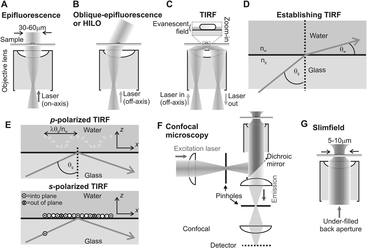
Figure 3.5 Different fluorescence illumination modes. (a) Wide-field epifluorescence using laser excitation. (b) Oblique epifluorescence or highly inclined and laminated optical sheet illumination. (c) Total internal reflection fluorescence (TIRF) using the objective lens method. (d) Schematic for refraction of a laser beam incident on a glass–water interface. (e) The E-field polarization vectors in the TIRF evanescent field generated during (A) p-TIRF excitation (incident polarization vector shown by small light-shaded arrow is in the plane of the page and the evanescent field polarization cartwheels across the surface) and (B) s-TIRF excitation (the incident polarization vector shown by small circle is into the plane of the page, and the axis of this polarization vector in the evanescent field remains parallel to this incident polarization, that is, conserved, though the polarization vector will also periodically extend both into and out of the plane of the page). (f) Confocal microscope schematic arrangement. (g) Slimfield illumination.
A laser beam can be tightly focused into the back aperture of an objective lens, unlike spatially extended sources such as arc lamps or LEDs, and so there is a room to translate the focus laterally away from the optic axis, allowing the angle of incidence to be adjusted. Beyond the critical angle, TIRF excitation is generated. However, an angle of incidence between zero and the critical angle results in oblique epifluorescence (Figure 3.5b), also known as variable-angle epifluorescence, oblique epi illumination, pseudo-TIRF, quasi-TIRF, near-TIRF, leaky TIRF, and highly inclined and laminated optical sheet illumination (HILO) (see Tokunaga et al., 2008). Oblique epifluorescence results in uniform excitation intensity parallel to the excitation field wave vector but has lower back scatter from cellular samples and from the surface of the microscope slide/coverslip, which can increase the contrast compared to standard epifluorescence by almost an order of magnitude.
3.6.2 Total Internal Reflection Fluorescence
TIRF microscopy (for a comprehensive discussion, see Axelrod et al., 1984) generates wide-field excitation laterally in the focal plane of a few tens of microns diameter but utilizes a near-field effect (i.e., an optical phenomenon over a length scale of less than a few wavelengths of light) parallel to the optic axis of the microscope objective lens to generate a fluorescence excitation field very close to a glass microscope slide/coverslip of ~100 nm characteristic depth (Figure 3.5c). TIRF is an enormously powerful and common biophysical technique, and so we cover several technical aspects of its use here. TIRF usually utilizes laser excitation, such that a beam of wavelength λ is directed at an oblique supercritical angle θ to the interface between a glass microscope coverslip and a water-based solution surrounding a biological sample. Total internal reflection of the incidence beam occurs at angles of incidence, which are greater than a critical angle θc:
(3.37)where nw and ng refer to the refractive indices of water (~1.33) and glass (~1.515, for commonly used BK7 low-fluorescence borosilicate glass), respectively, which indicates a critical angle of ~61°. These refractive index values relate to the wavelength-dependent dispersion relation of light, and across the VIS light spectrum of 400–700 nm result in a range of 1.344–1.342 (nw) and 1.529–1.514 (ng). The simplest empirical model for the dispersion relation is embodied in the Cauchy equation:
(3.38)The agreement with experiment in the VIS range is very good (within a few %), but larger inaccuracies exist beyond this range. A more accurate approximation comes directly from the classical solution to Maxwell’s equations for damped Lorentz oscillators, resulting in the Sellmeier equation:
(3.39)To understand how the evanescent field is generated, we can first apply Snell’s law of refraction, from glass to water (Figure 3.5d):
(3.40)where
- θg is the angle of incidence through the glass
- θw is the angle of refraction through the water
Thus, by rearrangement
(3.41)where b is a real number in the case of TIRF; thus the angle of refraction into the water is a purely imaginary number. The E-field in water in the 2D cross-section of Figure 3.3d can be modeled as a traveling wave with distance and wave vectors of magnitude r(x, z) and wave vector kw, respectively, with angular frequency ω after a time t, with z parallel to the optic axis of the objective lens and xy parallel to the glass–water interface plane:
(3.42)By substitution from Equation 3.41, we get the evanescent wave equation:
(3.43)The intensity I(z) of the evanescent field at x = 0 as a function of z (i.e., as it penetrates deeper into the solution) decays exponentially from the glass–water interface, characterized by the depth of penetration factor d:
(3.44)where
(3.45)A typical range of values for d is ~50–150 nm. Thus, after ~100 nm, the evanescent field intensity is ~1/e of the value at the microscope glass coverslip surface, whereas at 1 μm depth from the coverslip surface (e.g., the width bacteria), the intensity is just a few thousandths of a percent of the surface value. Thus, only fluorophores very close to the slide are excited into significant fluorescence, but those in the rest of the sample or any present in the surrounding solution are not. In effect, this creates an optical slice of ~100 nm thickness, which increases the contrast dramatically above background noise to permit single-molecule detection. It is possible to adjust the angle of incidence θg to yield d values smaller than 100 nm, limited by the numerical aperture of the objective lens (see Worked Case Example 3.1) and also larger values, such that d → ∞ as θg → θc.
The intensity of the evanescent field is proportional to the square of the E-field amplitude, but also depends on the polarization of the incidence E-field in the glass and has different values for the two orthogonal polarization components in water. Incident light that is polarized parallel (p) to the xz plane of incidence as depicted in Figure 3.5e generates an elliptically polarized evanescent field consisting of both parallel and perpendicular (s) polarized components. Solving Maxwell’s equations generates the full solutions for the electric field vector components of the evanescent field as follows:
(3.46)
where Ep,0 and Es,0 are the incident light E-field amplitudes parallel and perpendicular to the xz plane. As these equations suggest, there are different phase changes between the incident and evanescent E-fields parallel and perpendicular to the xz plane:
(3.49)
As these equations depict, the orientation of the polarization vector for s-polarized incident light is preserved in the evanescent field as the Ey component; as the supercritical angle of incidence gets closer to the critical angle, the Ex component in the evanescent field converges to zero and thus the p-polarized evanescent field converges to being purely the Ez component. This is utilized in the p-TIRF technique, which uses incident pure p-polarized light close to, but just above, the critical angle, to generate an evanescent field, which is polarized predominantly normal to the glass coverslip–water interface. This has an important advantage over subcritical angle excitation in standard epifluorescence illumination, for which the angle of incidence is zero, since in p-TIRF the polarization of the excitation field is purely parallel to the glass–water interface and is unable to excite a fluorophore whose electric dipole axis is normal to this interface and so can be used to infer orientation information for the fluorophore electric dipole axis. In the general case of supercritical angles not close to the critical angle, the p-polarized component in the evanescent field spirals elliptically across the spatial extent of the glass–water interface in a cartwheel fashion with a sinusoidal spatial periodicity of λ/nw sin θg (Figure 3.5f).
The intensity of both the p and s components in the evanescent field can both be several times greater than the incident intensity for values of θg between θc and ~75°–80°, with the p component marginally greater than the s component and then both tailing off to zero as θc → 90°:
(3.51)
Often, the incident E-field polarization will be circularized by a quarter-wave plate. The effect of a quarter-wave plate, similar to those utilized in phase contrast microscopy, is to retard the phase of any light whose polarization vector is aligned to the plate’s slow axis by one quarter of a wavelength relative to incident light whose polarization vector is aligned to the plate’s fast axis (90° rotated from the fast axis). If linearly polarized light is incident on the plate oriented at 45° to both the fast and slow axes, then circularly polarized light is generated such that the polarization vector of the light after propagating through the plate rotates around the wave vector itself with a spatial periodicity of one wavelength. The effect is to minimize any bias resulting from preferred linear polarization orientations in the absorption of the incident light from the relative orientation of the electric dipole moment of the fluorescent dye tag, but it should be noted that this does not result in a complete randomization of the polarization vector.
TIRF, in modern microscope systems, is generated either using a prism method or an objective lens method. The prism method results in marginally less undesirable incident light scattering than the objective lens method, since the light does not need to propagate across as many optical surfaces en route to the sample. However, fluorescence emissions need to be collected through the thickness of a microscope flow cell, ~100 μm depth filled with water; to avoid aberration effects normally requires the use of a special water-immersion objective lens to image through the bulk of the sample solution, which have a marginally lower numerical aperture (~1.2) than used for the objective lens method, and therefore the photon collection efficiency is lower. In Equation 3.45, the term ngsin θg is identical to the numerical aperture of the objective lens, and therefore to generate TIRF using the objective lens method requires an objective lens whose numerical aperture is greater than the refractive index of water, or ~1.33 (values of 1.4–1.5 in practice are typical).
The first application of TIRF to cellular investigation was to study epidermal growth factor (EGF) receptors in the cell membrane whose biological function is related to cell growth and development in the presence of other nearby cells (e.g., in a developing tissue) in which the EGF receptors were tagged with the cyanine dye Cy3 (Sako et al., 2000). Many biophysical investigations that use TIRF also utilize Förster resonance energy transfer (FRET). This is a nonradiative technique occurring over a nanometer length scale between two different dye molecules, and thus is a technique for investigating putative interaction of different biomolecules (discussed fully in Chapter 4). TIRF can also be combined with fluorescence polarization microscopy measurements for in vitro and cellular samples.
Several surface-based in vitro assays benefited from the enhancement in contrast using TIRF illumination. A good historical example in biophysics is the in vitro motility assay used to study molecular motors. This assay was designed to monitor the interaction of molecular motors that run on molecule-specific tracks, originally developed for observing muscle-based molecular motors. Here, F-actin filaments of several microns in length are conjugated with the fluorescent dye rhodamine and can be observed using TIRF in exceptional detail to undergo active diffusion on a microscope coverslip surface coated with the protein myosin in the presence of ATP due to the interaction between the molecular motor region of the myosin head domain with its F-actin track, as occurs in vivo in muscle, fueled by chemical energy from the hydrolysis of ATP (the theoretical model of this motor translocation behavior is discussed in Chapter 8).
Delimitation of light excitation volumes can also be achieved through the use of waveguides. Here, light can be guided through a fabricated optically transparent material, such as glass, to generate a supercritical angle of incidence between the waveguide surface and a physiological buffer containing a fluorescently labeled biological sample. This type of approach can be used to generate an evanescent field at the tip of an optical fiber, thus allowing fluorescence detection from the end of the fiber. This approach is used in nanophotonics, which enables complex shaped evanescent fields to be generated from fabricated waveguides, and has relevance toward enhancing the contrast of fluorescence detection in microfluidics-based biosensing devices (see Chapter 7).
3.6.3 Fluorescence Polarization Microscopy
Fluorescence polarization measurements can be performed by adapting a standard fluorescence microscope to split the orthogonal emission polarization onto either two separate cameras, or potentially onto two halves of the same camera pixel array in a similar manner to splitting the fluorescence emissions on the basis of wavelength except using a polarization splitter optic instead of a dichroic mirror. Typically, the incident E-field polarization is fixed and linear, but as discussed in the previous section, standard epifluorescence illumination is suitable since it results in excitation polarization parallel to the microscope coverslip or slide.
It is also possible to apply polarization microscopy using TIRF illumination. If the incident light onto the glass–water interface is purely s-polarized, then the polarization orientation will be conserved in the evanescent excitation. However, as discussed, useful information can also be obtained by using p-polarized excitation light for TIRF, that is, p-TIRF. Here, the polarization vector is predominantly normal to the glass–water interface, and so has application in monitoring fluorophores whose electric dipoles axes are constrained to be normal to a microscope coverslip; an example of such is for voltage-sensitive membrane-integrated dyes.
The cartwheeling polarization vector of the p component of the evanescent excitation field in the general case of supercritical angle TIRF results in a well-characterized spatial periodicity of a few hundred nanometers. This is a comparable length scale to some localized invaginations in the cell membrane called “caveolae” that may be involved in several different biological processes, such as environment signal detection, and how large particles enter eukaryotic cells including food particles through the process of endocytosis, how certain viruses infect cells, as well as how particles are secreted from eukaryotes through the process of exocytosis (see Chapter 2). Using specialized membrane-permeable fluorescent dyes that orient their electric dipole axis perpendicular to the phospholipid bilayer plane of the cell membrane, p-polarization excitation TIRF microscopy can be used to image the spatial architecture of such localized membrane invaginations (Hinterdorfer et al., 1994; Sund et al., 1999).
3.6.4 Confocal Microscopy
An in vivo sample in a light microscope can often encapsulate a height equivalent to tens of equivalent depth of field layers, which can generate significant background noise on the image. The most robust standard biophysical tool to limit this effect is that of confocal microscopy, which uses a combination of two pinholes, in front of the sample and the detector (Figure 3.5g) to delimit the detected intensity to that emerging from the focal plane, resulting in significant increases in fluorescence imaging contrast. Laser light is focused to a volume of just 1 femtoliter (fL), 10−18 m3, onto the sample that is either raster scanned across the sample or the sample stage raster scanned relative to the laser focus. Fluorescence emissions acquired during the analog raster scanning are then digitized during software reconstruction to create a 2D pixel array image.
The confocal volume can be approximated as a 3D Gaussian shape, roughly like an egg, with its long vertical axis parallel to the microscope optic axis that is longer than the lateral width w in the focal plane by a factor of a of typically ~2.5, giving a volume V:
(3.53)Photon emissions are ultimately focused onto a sensitive detector, typically a PMT, which can then be reconstituted from the raster scan to form the 2D image. Slow speed is the primary disadvantage, limited to ~100 fps. Improvements have involved high-speed spinning disk (or Nipkow disk) confocal microscopy comprising two coupled spinning disks scanning ~1000 focused laser spots onto a sample at the same time allowing imaging of ~1000 fps. The principal issue with such fast confocal imaging methods is that the extra exposure to light can result in significant photodamage effects on living biological samples.
The lateral width w is determined by the PSF of the microscope. Note that this value is identical to the optical resolution limit in diffraction-limited light microscopy, discussed fully in Chapter 4. For a circular aperture objective lens of numerical aperture NA:
(3.54)For determining the excitation volume size in confocal imaging, this formula can be also used with the radius of the confocal volume in the focal plane equal to w. For determining the resolution of the fluorescence emission images for VIS light fluorescence, the wavelength λ is normally in the range 500–700 nm, low-magnification light microscopy allows fields of view of several hundred microns or more in diameter to be visualized in a single image frame, w can be as low as 1–2 μm (essentially the length scale of subcellular organelles in a eukaryotic tissue, or single bacterial cells within a biofilm), whereas the highest magnification light microscopes have the smallest values of w of ~250–300 nm. The Nyquist criterion indicates that pixel edge length in a digitized confocal microscopy image should be less than half the size of the smallest resolvable length scale, that is, w/2, in the sample to overcome undersampling, and in practice, pixel edge lengths equivalent to 50–100 nm in the sample plane are typical.
The axial spatial resolution in confocal microscopy is worse than the lateral resolution w by the same factor of ~2.5 for the relative stretching of the PSF parallel to optic axis to generate a roughly ellipsoidal volume. A modification to standard confocal imaging is used in confocal theta microscopy in which juxtaposed confocal volumes are angled obliquely to each other (ideally perpendicularly) to interfere at the level of the sample that generates a reduced size of confocal volume with a resultant small improvement to axial resolution.
The z range of confocal microscopy illumination is sometimes limited by diffractive effects of the confocal beam. The standard illumination intensity of a confocal microscope laser beam incident on the back aperture of the objective lens has a Gaussian profile, resulting in a divergent confocal volume that, as we have seen, has an aspect ratio parallel to the optic axis of ~1:3, implying that a wide area of sample can obstruct the incident beam en route to the focal waist if imaging reasonably deep into a large cell or multicellular tissue sample. The use of Bessel beam illumination can circumvent this problem. A Bessel beam is nondiffractive (discussed fully, in the context of their application in OTs, in Chapter 6), which means that it is relatively nondivergent and insensitive to minor obstructions in the beam profile. A Bessel beam can be used as an alternative source of scanning illumination for exciting fluorophores in the sample (see Planchon et al., 2011), but note that since the beam is nondivergent the ability to optically section in z is much reduced compared to standard confocal microscopy.
Another application of confocal illumination is to monitor the diffusion of biomolecules in tissues, or even single cells. This can be achieved using the technique of fluorescence recovery after photobleaching (FRAP). Here, a relatively intense confocal excitation volume is generated for the purpose of photobleaching dye molecules of a specific fluorescently labeled biomolecule in that region of space. If the laser intensity is high enough, then relatively little diffusion will occur during the rapid photobleach process. Before and after imaging in fluorescence then shows a dark region indicative of this photobleaching. However, if subsequent fluorescence images are acquired, then fluorescence intensity may recover in this bleached region, which is indicative of diffusion of photoactive dye-labeled biomolecules back into this bleached area. This can be used to determine rates of diffusion of the biomolecule, but also rates of biomolecule turnover in distinct molecular complexes (see Chapter 8).
A related technique to FRAP is fluorescence loss in photobleaching (FLIP). This experimental photobleaching method is similar, but fluorescence intensity measurements are instead made at positions outside of the original bleach zone. Here, the diffusion of photobleach dye-labeled biomolecules results in a decrease in fluorescence intensity in surrounding areas. FLIP gives similar information to FRAP but can also yield more complex features of heterogeneous diffusion between the point of photobleaching and the physically distant point of fluorescent intensity measurement.
3.6.5 Environmental Fluorescence Microscopy
Fluorescence microscopy can be adapted to provide information about the local physical and chemical environment in the vicinity of a fluorescent dye label. For example, confocal microscopy can be utilized to probe the intracellular environment by precise measurement of the lifetime of a fluorophore attached to a specific biological molecule using a technique called FLIM, which is spatially dependent upon physical and chemical parameters such as the local pH and the concentration of certain ions, especially chloride (Cl−). The lifetime of the excited fluorescence state typically varies in the range 10−9 to 10−7s and can be measured by synchronizing the fluorescence detection to the excitation using a rapidly pulsed laser at least tens of megahertz frequency. Usual confocal-type imaging is applied with lateral xy scanning of the sample through the confocal volume resulting in a 2D map of fluorescence lifetimes across the extent of the cell, unlike conventional fluorescence imaging that generates maps of fluorescence intensity. Confocal microscopy allows images at different values of height z to be generated, thus in principle enabling the fluorescence lifetime volume in a cell to be reconstructed. The same principle can also be used applying multiphoton excitation to further improve the spatial resolution.
The fluorescence lifetime can be expressed as the reciprocal of the sum of all the rate constants for all the different fluorescence decay processes present. It can be measured using either a frequency or time domain method. For the time-domain method, a high-bandwidth detector such as an APD or PMT is used to perform time-correlated single-photon counting (TCSPC) to count the arrival time of a photon after an initial laser excitation pulse. To improve sampling speed, multiple detection (usually in the range 16–64) can be employed.
The arrival times are modeled as a Poisson distribution, and after this process is repeated several times, sufficient statistics are acquired to estimate the fluorescence lifetime from binned arrival time histograms using an exponential fit. Some older FLIM equipment still in operation use instead a gating optical intensifier that is only activated after a small proportion of the fluorescence light is directed onto a photodiode via a dichroic mirror, such that photon detection is only possible after a programmed electronic delay. By performing detection across a range of delay times thus similarly allows the fluorescence lifetime to be estimated, but with poorer time resolution compared to TCSPC and lower photon collection efficiency.
For the frequency domain approach, the fluorescence lifetime is estimated from the phase delay between a high-frequency modulated light source such as an LED or laser modulated using an AOD (see Chapter 6), coupled to a fast intensified camera detector. An independent estimate of the lifetime may also be made from the modulation ratio of the y components of the excitation and fluorescence. If these values do not agree within experimental error, it may indicate the presence of more than one lifetime component. Frequency domain methods are faster than time domain approaches due to the use of camera detection over slow lateral scanning, and thus are the most commonly used for dynamic cellular studies.
Molecular interactions may also be monitored by using a variant of the technique called FLIM–FRET. This technique utilizes the fact that the lifetime of a fluorophore will change if energy is non-radiatively transferred to, or from it, from another fluorophore in a very close proximity via FRET. Separate lifetime measurements can be made on both the FRET donor dye at shorter wavelengths and FRET acceptor dye at longer wavelengths (FRET effects are discussed fully in Chapter 4) to infer the nanoscale separation of two different biological molecules separately labeled with these two different dyes. FLIM–FRET therefore can generate cellular molecular interaction maps.
Also, a range of fluorophores are now available whose fluorescence lifetime is dependent on the local viscosity of their cellular environment (Kuimova, 2008). These dye molecules typically operate by undergoing periodic mechanical transitions as nanoscale rotors in forming a transient electrical dipole that can absorb excitation light. As with all dyes, each molecule will emit a characteristic approximate number of photons prior to irreversible photobleaching most likely due to free radical chemical damage of the dye. Since the frequency of rotation of the dye is a function of local viscosity, the dye fluorescence lifetime is therefore a metric for viscosity, and thus FLIM measurements using such dyes can map out viscosity over single cells. This is important since local cellular viscosity is a manifestation of the underlying subcellular architecture in that specific region of the cell and thus gives us insight into these different biological features at the nanoscale.
There are also several fluorophores available whose fluorescence emission output is particularly sensitive to specific chemical and physical environmental conditions. Into this category can be included voltage-sensitive dyes and probes which can measure molecular crowding (for example, a FRET pair of fluorescent protein molecules attached by a lever arm which closes to give high FRET efficiency at high molecular crowding conditions but opens out to give a lower FRET efficiency at low molecular crowding. But other dyes also exist, which have been chemically optimized to be highly sensitive to local pH or the binding of ions such calcium (Ca2+), whose fluorescence intensity and fluorescence lifetime change in response to binding. These dyes therefore act as nanoscale environmental sensors, and FILM can map out the absolute values of these environmental parameters in the cell. Many of these dyes operate through having specific regions of their emission spectra, which are sensitive to environmental change, whereas other regions of the emission spectrum may be relatively insensitive. Usually, therefore, a ratiometric approach is taken to measure the relative ratio of emission intensity change at the sensitive and insensitive regions of the emission spectrum, since this ratio will no longer be sensitive to absolute concentrations of the dye in a given localization of the cell.
Direct measurement of the integrated fluorescence intensity of individual dye molecules can also be used as a metric for the physical and chemical environment, that is, the total brightness of a dye molecule is a function of several different environment factors, depending upon the specifics of the dye. A more precise metric is to perform spectral imaging of the dye molecule. Here, the fluorescence emission signal can be directed through a transmission diffraction grating, such that the zeroth order (undeviated light) can be imaged onto one-half of a camera detector, while the first order (deviated light) is imaged onto the other half. The zeroth order can be used to determine precisely where the molecule is by using localization fitting algorithms (discussed in Chapter 4) while the first order is a measurement of the transmission spectrum of that dye molecule, since the diffraction angle is wavelength dependent. Thus, the 1D profile of this spectral image can therefore be used as a very precise indicator for local environmental parameters.
3.6.6 Slimfield and Narrow-Field Epifluorescence Microscopy
Biological molecules typically diffuse much faster inside the watery innards of cells than in membrane surfaces due to lower effective viscosities in the cell cytoplasm by two to three orders of magnitude, and they have a high likelihood of moving during each sampling time window for slow scanning techniques and thus are too blurred to monitor their localization in a time-resolved fashion (i.e., it is not possible to track them). To beat the blur time of biomolecules requires imaging faster than their characteristic diffusional time.
In a sampling time window Δt, a molecule with effective diffusion coefficient D will diffuse a root mean squared displacement √〈R2〉 of √(2DnΔt) (see Equation 2.12) in n-dimensional space. To estimate what maximum value of Δt we can use in order to see a fluorescently labeled molecule unblurred, we set √〈R2〉 equal to the PSF width. Using this simple assumption in conjunction with the Stokes–Einstein relation (Chapter 2) it is trivial to derive:
(3.55)where λpeak is the peak fluorescence emission wavelength through an objective lens of numerical aperture NA of a fluorescent-labeled molecule of effective Stokes radius rStokes diffusing in a medium of viscosity η. For typical nanoscale globular biomolecules for a high-magnification fluorescence microscope, this indicates a maximum sampling time window of a few hundred milliseconds for diffusion in cell membranes (2D diffusion), and more like a few milliseconds in the cytoplasm (3D diffusion). Thus, to image mobile molecular components inside cells requires millisecond time resolution. Note that if the fluorophore-labeled biomolecule exhibits ballistic motion as opposed to diffusive motion (e.g., in the extreme of very short time intervals that are less than the mean collision time of molecules in the sample), then the root mean squared displacement will scale linearly with Δt as opposed to having a square root dependence, thus requiring a shorter camera sampling time window than Equation 3.55 suggests.
However, the normal excitation intensities used for conventional epifluorescence or oblique epifluorescence generate too low a fluorescence emission signal for millisecond sampling, which is swamped in camera readout noise. This is because there is a limited photon budget for fluorescence emission and carving this budget into smaller and smaller time windows reduces the effective signal until it is hidden in the noise. To overcome this, the simplest approach is to shrink the area of the excitation field, while retaining the same incident laser power, resulting in substantial increases in excitation intensity. Narrow-field epifluorescence shrinks the excitation intensity field to generate a lateral full width at half maximum of ~5–15 μm, which has been used to monitor the diffusion of single lipid molecules with millisecond time resolution (Schmidt et al., 1996), while a variant of the technique delimits the excitation field by imaging a narrow pinhole into the sample (Yang and Musser, 2006).
A related technique of Slimfield microscopy generates a similar width excitation field in the sample but achieves this by propagating a narrow collimated laser of width ws (typically <1 mm diameter) into the back aperture of a high NA objective lens resulting in an expanded confocal volume of lateral width wc, since there is a reciprocal relation in Gaussian optics between the input beam width and output diffraction pattern width (see Self, 1983):
(3.56)where f is the focal length of the objective lens (typically 1–3 mm). Since the Slimfield excitation is a confocal volume and therefore divergent with z away from the laser focus, there is some improvement in imaging contrast over narrow field in reducing scattering from out-of-focus image planes.
The large effective excitation intensities used in narrow-field and Slimfield approaches result in smaller photobleach times for the excited fluorophores. For example, if the GFP fluorophore is excited, then it may irreversibly photobleach after less than a few tens of milliseconds, equivalent to only 5–10 consecutive image frames. This potentially presents a problem since although the diffusional time scale of biomolecules in the cytoplasm is at the millisecond level, many biological processes will typically consist of reaction–diffusion events, characterized by fast diffusion of one more molecular component but often slow reaction events with other components (see Chapter 8). Thus, the time scale for the entire process may be substantially longer than the millisecond diffusional time scale. To overcome this issue, individual millisecond image frames may be obtained discontinuously, that is, using strobing. In this way, the limited fluorescence emission photon budget of a single fluorescent protein molecule may be used over substantially longer time scales than just a few tens of milliseconds to gain insight into the dynamics of several different processes inside the cell while still enabling unblurred fluorophore detection on individual images frames. A technical issue in regard to strobing is the bandwidth of the shuttering mechanism used to turn the laser excitation on and off. Typical mechanical shutters are limited to a bandwidth of ~100 Hz, and so the minimum sampling time window that can be accommodated is ~10 ms, which is too high for millisecond imaging. Alternative faster shuttering can be implemented directly through electronic modulation of the laser power output on some devices or utilizing acousto-optic-based technology for shuttering, for example, an acousto-optic modulator that can be shuttered at >MHz bandwidth using similar physics principles to AODs (see Chapter 6).
3.7 Summary Points
- Elastic scattering light spectroscopy—using VIS light, UV, and IR—is a robust tool to determine the concentration of biological scattering particles in solution.
- Fluorescence spectroscopy and FACS can characterize and help isolate different cell types.
- Image contrast can be improved in bright-field microscopy using a range of tools, especially those involving optical interference, which includes phase contrast and DIC microscopy.
- Single-photon excitation fluorescence microscopy is one of the most widely used and valuable biophysical tools to investigate functional biological material, especially when combined with multiple color dye tags.
- Of the many different types of dye tags used in fluorescence microscopy, FPs offer the greatest physiological insight but have suboptimal photophysical features and often cause steric hindrance of native biological functions.
- There are several different modes of illumination for fluorescence microscopy, from which TIRF offers huge enhancements in contrast for monitoring processes in cell membranes in particular.
Questions
- 3.1 Give an example of how a biological process spans multiple length and time scales and crosses over and feedbacks at several different levels of length and time scale. Describe an experimental biophysical technique that can be used to generate information potentially at the whole organism, single-cell, and single-molecule levels simultaneously. Should we try to study even broader length and time scales regimes, for example, at the level of ecosystems at one end of the spectrum or quantum biology at the other? Where should we stop and why?
- 3.2 Transmission electron microscopy (see Chapter 5) on a layer of cells in a tissue suggested their nuclei had mean diameters of 10.2 ± 0.6 μm (± standard deviation). Negative-phase contrast microscopy images from this tissue suggested that the nuclei were the brightest features in the image when the nuclei were most in focus.
- Derive a relation between the length through a cell over which the phase of propagating light is retarded by one quarter of a wavelength, stating any assumptions.
- Estimate the range of refractive index for the nuclei.
- 3.3 What do we mean by an isotropic emitter in the context of a fluorescent dye molecule? Derive an expression relating the geometrical efficiency of photon capture of an objective lens of numerical aperture (NA) (i.e., what is the maximum proportion of light emitted from an isotropic emitter, neglecting any transmission losses through the lens). What factors may result in fluorescence emission not being isotropic?
- 3.4 Fluorescence anisotropy experiments were performed on a GFP-tagged protein in aqueous solution, whose effective Stokes radius was roughly twice that of a single GFP molecule. Estimate what the minimum sampling frequency in GHz on the photon detector needs to be to detect anisotropic emission effects. (Assume that the viscosity of water is ~0.001 Pa·s.)
- 3.5 The same protein of Question 3.3 under certain conditions binds to another protein in the cell membrane with the same diameter, whose length spans the full width of the membrane. If this GFP-tagged protein is imaged using a rapid sampling fluorescence microscope, which can acquire at a maximum sampling time of 1000 image frames per second, comment on whether it will be possible to use fluorescence polarization images to determine the state of the membrane protein’s angular rotation in the membrane.
- 3.6 A yellow FP called “YPet,” at peak emission wavelength ~530 nm, was used to tag a low copy number cytoplasmic protein in a spherical bacterial cell of radius ~1 μm. A slimfield microscope, using an objective lens of NA 1.45 with EMCCD camera detector with pixel edge length 18.4 μm and a magnification of 300 between the sample and the camera, was used to monitor the localization of the protein with millisecond sampling, suggesting the protein was freely diffusing with a mean of two fluorescent spots detected at the start of each acquisition if the focal plane of the microscope was set to the midpoint of each cell. Estimate the intracellular concentration in nanomolar of the protein.
- 3.7 What do we mean by the Stokes shift, and where does it originate from? Why does the normalized excitation spectrum of a fluorophore look like a rough mirror image of the normalized emission spectrum?
- 3.8 A fluorescence microscopy experiment using an objective lens of numerical aperture 0.9 was performed on a zebrafish embryo (a “model organism” used to investigate multicellular tissues, see Chapter 7) to investigate a single layer of GFP-labeled cells of 10 μm diameter, focusing at the midheight level of the cells. These cells were expected to express a mean number of 900 GFP-tagged protein molecules per cell with a standard deviation of 500 molecules per cell. Typical cells had a measured intensity during fluorescence microscopy of ~107 counts per cell integrated over the whole of the data acquisition prior to cells being completely photobleached. Data were acquired from a high-efficiency camera detector whose magnification per pixel was equivalent to 200 nm at the sample, gain was 300. Similar cells from another zebrafish in which there was no GFP had a total measured intensity during the same fluorescence microscopy imaging of ~2 × 10⁶ counts.
- Assuming that captured fluorescence emissions come from a cell slice whose depth is equivalent to the depth of field of the objective lens, estimate the number of fluorescence emission photons detected from a single molecule of GFP.
- The quantum efficiency of the camera was ~90%, the transmission function of the dichroic mirror transmits a mean of 85% of all GFP fluorescence emissions, and an emission filter between the dichroic mirror and camera transmits 50% of all GFP fluorescence emissions. The transmission losses due to other optical components on the emission pathway of the microscope resulted in ~25% of all light not being transmitted. Estimate the mean number of photons emitted in total per GFP molecule, stating any assumptions.
- 3.9 A similar experiment was performed on the cells from Question 3.5, but on a thicker tissue section 80 μm thick, consisting of a 70 μm layer of similar cells not labeled with GFP close to the microscope’s coverslip surface, above which are the single layer of GFP-labeled cells.
- Assuming that the rate at which light is absorbed when it propagates through a homogeneous tissue is proportional to its intensity and to the total number of molecular absorption event, derive the Beer–Lambert law, stating any assumptions.
- If each layer of cells attenuates, the excitation beam by 4% calculates the total integrated emission signal due to GFP from a single cell using the same microscope and camera detector and of focusing at mid-cell height for the GFP-labeled cells, acquiring data until the cells are completely photobleached as before.
- Estimate the total noise per cell detected during these data acquisitions.
- To detect a given cell reliably above the level of noise, the effective SNR needs to be above ~2. If the tissue area is ~100 × 100 μm, estimate how many cells you would expect to detect, stating any assumptions you make.
- 3.10 Describe the technique of TIRF microscopy and give an example of its application in biophysics. Most TIRF in vivo studies investigate membrane complexes; why is this? Would TIRF still be effective if there was a high concentration of auto-FPs in the cytoplasm? Can TIRF be applied to monitoring the nucleus of cells?
- 3.11 The wave equation for a plane wave of light has solutions of the form
- For real angles θ, this represents a traveling wave in the focal xy plane of the sample.
- Show that the same solution but with complex θ describes the electric field in water near a water–glass interface in the case where plane wave illumination is totally internally reflected within the glass at the interface.
- Obtain an expression in terms of the angle of incidence in glass, angular frequency ω, and the refractive indices of glass and water, for the electric field in water for the aforementioned case. Describe using a sketch the wave that this represents.
- 3.12 Does TIRF illumination require a coherent laser source, or would a noncoherent white-light source be okay?
- 3.13 A fluorescence imaging experiment was performed at video rate on a bespoke inverted microscope using Escherichia coli bacteria that have a shape close to a cylinder of length 2 μm capped by hemispheres of diameter 1 μm, in which a diffused cell membrane protein was tagged using GFP, with biochemical assays suggesting 200 proteins per cell, using a simple flow cell that consists of a glass coverslip in optical contact with a high numerical aperture objective lens via immersion oil, with a cell stuck to the coverslip surface in a water-based buffer, with the walls of the flow cell being 120 μm high stuck on the upper side to a glass microscope slide, above which was then simply air. The cells were first imaged using epifluorescence in which the emergent 473 nm laser excitation beam traveled from below and then straight up through the sample, resulting in a halolike appearance in fluorescence to cells that were stuck with their long axis parallel to the glass coverslip surface (a bright fluorescence at the perimeter of the cell when setting the focal plane to be at the midpoint of the cylinder).
- Explain these observations. The angle of incidence of the excitation beam was then increased from zero (epifluorescence), which resulted in the beam emerging from the top of the microscope slide at increasingly shallow angles. Eventually, the emergent beam angle was shallow enough that it just dipped below the horizon and could not be seen exiting the microscope slide. At that point, the experimentalists concluded that the system was set for TIRF imaging. However, they were surprised to still see a halolike appearance to the fluorescence images of the cells when they had expected to see a brighter region that marked the cell body.
- Explain these observations. (Hint: think about the microscope slide as well as the coverslip.)
- 3.14 A confocal microscopy experiment is performed where the focused laser volume had a lateral width measured at 230 nm and an axial width measured at 620 nm. Bacteria in the sample were rodlike with end-to-end micron length and 1 μm width, shaped like a cylinder capped at either end by a hemisphere, and contained a GFP-tagged protein in their cytoplasm.
- How much of a typical cell is excited by the confocal volume?
- If the focused laser beam is occupied by a single GFP-tagged protein in the cytoplasm of the cell for 50% of the time, what is the molarity of that protein? The laser beam is focused on to the cell’s midpoint in the cytoplasm. From measurements of GFP-tagged proteins diffusing through the confocal volume of fluorescence pulses from a few fluorescently tagged molecules, the range of time taken to traverse the confocal spot in the sample plane was estimated at 1.7 ± 0.7 ms.
- Estimate the effective diameter of the protein, stating any assumptions you make. (Assume that the viscosity of the cytoplasm in this case is ~0.002 Pa⋅s.)
- 3.15 An epifluorescence microscope with oil immersion (refractive index =1.515) objective lens NA 1.4, focal length 2 mm, was used to monitor a dye called Hoerchst, fluorescence emission peak wavelength 454 nm, which labels the DNA in a single rod-like E. coli bacterium lying flat with its long axis (length 3 µm, width 1 µm) on a coverslip. The downstream imaging path after the objective lens comprised a focal length 200 mm lens that makes a telescope with the objective lens, and another telescope with lenses of focal lengths 50 mm and 200 mm, which images onto a CMOS camera with pixel size 20 µm. 3D fluorescence imaging suggested that the width of the nucleoid was 0.48 µm. If a fluorescently tagged DNA binding protein bound transiently to the “bottom” region of the nucleoid closest to the coverslip but then diffused through the nucleoid and subsequently emerged from the ‘top’ nucleoid region furthest away in right from the coverslip, would you be able to track the protein for the entirety of this journey? (see Worked Case Example 8.4 for a related question.)
References
Key Reference
- Axelrod, D. et al. (1984). Total internal reflection fluorescence. Annu. Rev. Biophys. Bioeng. 13:247–268.
More Niche References
- Allen, K.N., and Imperiali, B. (2010). Lanthanide-tagged proteins—An illuminating partnership. Curr. Opin. Chem. Biol. 14:247–254.
- Corry, B. et al. (2006). Determination of the orientational distribution and orientation factor for transfer between membrane-bound fluorophores using a confocal microscope. Biophys. J. 91(3):1032–1045.
- Fara, P. (2009). A microscopic reality tale. Nature 459:642–644.
- Hinterdorfer, P. et al. (1994). Reconstitution of membrane fusion sites. A total internal reflection fluorescence microscopy study of influenza hemagglutinin-mediated membrane fusion. J. Biol. Chem. 269:20360–20368.
- Hooke, R. (1665). Micrographia: Or Some Physiological Descriptions of Minute Bodies Made by Magnifying Glasses with Observations and Inquiries Thereupon. Royal Society, London, U.K. Scanned manuscript from 1754 available at http://lhldigital.lindahall.org/cdm/ref/collection/nat_hist/id/0.
- Hughes, B.D., Pailthorpe, B.A., and White, L.R. (1981). The translational and rotational drag on a cylinder moving in a membrane. J. Fluid. Mech. 110:349–372.
- Kuimova, M.K. et al. (2008). Molecular rotor measures viscosity of live cells via fluorescence lifetime imaging. J. Am. Chem. Soc. 130(21):6672–6673.
- Marriott, G. et al. (2008). Optical lock-in detection imaging microscopy for contrast-enhanced imaging in living cells. Proc. Natl. Acad. Sci. USA 105:17789–17794.
- Michalet, X. et al. (2005). Quantum dots for live cells, in vivo imaging, and diagnostics. Science 307:538–544.
- Nasse, M.J. et al. (2011). High-resolution Fourier-transform infrared chemical imaging with multiple synchrotron beams. Nat. Methods 8:413–416.
- Piston, D.W. (2010). Fluorescence anisotropy of protein complexes in living cells. Biophys. J. 99(6):1685–1686.
- Planchon, T.A. et al. (2011). Rapid three-dimensional isotropic imaging of living cells using Bessel beam plane illumination. Nat. Methods 8:417–423.
- Popescu, G. (2011) Quantitative Phase Imaging of Cells and Tissues, McGraw-Hill, New York.
- Saffman, P.G. and Delbrück, M. (1975). Brownian motion in biological membranes. Proc. Natl. Acad. Sci. USA 72(8):3111–3113.
- Sako, Y. et al. (2000). Single-molecule imaging of EGFR signalling on the surface of living cells. Nat. Cell Biol. 2:168–172.
- Schmidt, T. et al. (1996). Imaging of single molecule diffusion. Proc. Natl. Acad. Sci. USA 93:2926–2929.
- Self, S.A. (1983). Focusing of spherical Gaussian beams. Appl. Opt. 22:658–661.
- Sund, S.E. et al. (1999). Cell membrane orientation visualized by polarized total internal reflection fluorescence. Biophys. J. 77:2266–2283.
- Tokunaga, M. et al. (2008). Highly inclined thin illumination enables clear single molecule imaging in cells. Nat. Methods 5:159–161.
- van Leeuwenhoek, A. (1702). Part of a letter from Mr Anthony van Leewenhoek, F.R.S., concerning green weeds growing in water, and some animalcula found about them. Philos. Trans. 23:1304–1311.
- Yang, W. and Musser, S.M. (2006). Visualizing single molecules interacting with nuclear pore complexes by narrowfield epifluorescence microscopy. Methods 39:316–328.